This page was last revised for version 5.1.0.
Fully automated tracing routines can be accessed through the Auto-trace menu in the main dialog.
Grayscale Images
Grayscale images are processed using the Auto-trace › Grayscale Image… command for single-cell tracing of images already loaded, or Auto-trace › Grayscale Image (Multiple Cells)… when the image contains multiple cells (see Multiple Cells). File-based and batch variants are available under Auto-trace › Batch Processing (Batch Processing).
This command reconstructs neuronal structures directly from grayscale (intensity) images without requiring binarization. The method is particularly effective for fluorescence microscopy images with bright foreground structures on dark backgrounds. It builds on two foundational algorithms: APP2 (Gray-Weighted Distance Transform with Fast Marching and hierarchical pruning) and neuTube (several of the post-processing refinements described below). SNT extends these with its own capabilities:
-
Images parsed at full-resolution and native bit-depth without downsampling
-
Big data support: Ability to process TB datasets that exceed available RAM
-
Learning from manual annotations: Ability to derive tracing parameters automatically from ground-truth paths, reducing trial-and-error when tuning the algorithm for a new dataset
-
Score maps for pruning guidance: Ability to use either Vesselness-based (e.g., Tubeness/Frangi) or external segmentation p-maps to better guide the detection of neurites
-
Tip extension across dim gaps: Ability to ‘hop’ over blebbed or non-contiguous signal
-
Post-hoc fitting for node position and radius refinement: Ability to obtain more natural curvatures by snapping traces to the neurite’s signal
-
Automated detection of somata: Ability to simultaneously seed the tracing algorithm on somata in a multi-cell labeled neuropil
-
Territory-controlled multi-soma tracing: Ability to predict whether a neurite belongs to which cell in a sparsely labeled multi-cell neuropil
For technical implementation details and references, see the SNT technical notes.
You can follow these instructions using File › Load Demo Dataset… and choosing either 1) the Drosophila OP neuron, a Drosophila olfactory projection neuron and respective ground truth reconstruction (single cell); or the Microglia cells dataset, a 2D image with multiple ramified microglia in the mouse retina.
Input Image
Grayscale Image (Mandatory) The intensity image to be traced (2D or 3D). Either the image currently loaded in SNT, or a Secondary image layer. Should contain bright neuronal structures on a dark background.
Soma/Root Detection
The algorithm requires a starting point (seed) to begin tracing. Several strategies are available:
-
None. Use auto-detection Automatically detects the soma/root at the thickest and brightest region as per Soma Detection. No ROI is required
-
Area ROI around soma: One tree per primary neurite An area ROI delineates the soma boundary. Creates separate trees for each neurite exiting the soma, rooting them at the soma perimeter. Best for complex morphologies where multiple primary branches emerge from the cell body and individual neurites need to be analyzed separately
-
Single tree rooted at ROI centroid The ROI marks the soma location. Creates a single tree rooted at the geometric centroid of the ROI. Suitable for simple morphologies or when the entire arbor should be represented as one connected structure
-
Single tree rooted at ROI weighted centroid Similar to the above, but roots the tree at the intensity-weighted centroid of nodes traced within the soma region, rather than the ROI’s geometric center. More accurate when the ROI encompasses the entire soma but may not be precisely centered
When working with 3D images, the Active plane only option restricts the ROI to its specific Z-slice, preventing the algorithm from considering roots at other depths.
")
Thresholding
Background threshold Defines the intensity cutoff below which pixels are considered background and excluded from tracing. Lower values trace more structures (including noise), while higher values trace less (potentially missing dim neurites).
- Use
-1(default) for automatic threshold estimation using image statistics - Adjust manually if auto-detection includes too much noise or misses dim structures
- Valid range: -1 (auto) to the image maximum intensity
Branch Filtering and Scoring
These parameters control which branches are retained in the final reconstruction:
Score map filter Selects a vesselness filter used to compute a confidence map for each traced segment. The score map assigns a “how tube-like is this location” score to every node, enabling adaptive pruning that adapts to each segment’s minimum radius: The pruning is more lenient for thin structures and stricter for thick ones. Options include:
- None: Disables score-based pruning
- Tubeness (default): Hessian-based tubeness filter, computed at scales derived from the radius distribution (25th/50th/75th percentile) of the initial reconstruction
- Frangi: Frangi vesselness filter, an alternative Hessian-based approach
- Secondary image layer: Uses the currently loaded secondary layer as a pre-computed score map (e.g., a deep-learning probability map obtained outside SNT)
Min. branch score The minimum intensity-weighted score threshold for branches to be included. This metric accumulates normalized pixel intensities along each branch path (rather than measuring spatial distance), so brighter branches accumulate score faster than dim ones. Branches below this threshold are pruned as noise. Increase to remove small spurious branches; decrease to retain finer details. Default: 5.0
Branch sensitivity Controls how aggressively dim branches are pruned relative to the overall signal. Higher values impose stricter requirements; lower values are more permissive. Default: 0.3
Overlap tolerance Controls overlap detection between traced branches and existing structures. Higher values allow more overlap before a branch is pruned. Default: 0.1
Strict tip filtering When enabled, removes terminal branches that substantially overlap with their parent branch. Useful for eliminating false-positive branches that shadow thick parent neurites. Default: off
Post-processing
After the initial tree extraction and branch filtering, several post-processing steps refine the geometry and topology of the reconstruction:
Max. branching angle Controls branch-point parent reassignment (branch tuning). At each branch point, the algorithm tests whether re-attaching a continuation node to its grandparent or a sibling produces a straighter path. If the alternative attachment avoids a turn exceeding the specified angle, the topology is rewired. Set to -1 to disable. Default: 90°
Tip extension distance (voxels) Maximum distance (in voxels) for A-based tip extension (experimental feature). After pruning, each leaf tip is scanned along its tangent direction for bright signal beyond the Fast Marching frontier. If a foreground target is found within this distance, an A path is traced through the gap and grafted onto the tree. Each candidate bridge is validated against geometric and intensity criteria (contraction ratio, direction compatibility, mean intensity). Disconnected components that cannot be bridged are discarded. Set to 0 to disable. Default: 0 (disabled)
Remove zigzags When enabled (default), iteratively detects and collapses zigzag artifacts: consecutive nodes that both form sharp turns (angles of 90°—270°). The inner node is merged into its parent. The process repeats until no more zigzags are found, producing smoother paths at junctions
Remove overshoots When enabled (default), detects and removes overshoot nodes in a single pass. A node is an overshoot if it forms a sharp turn and exactly one of its neighbors (parent or child) is a branch point. Such nodes likely represent tracing artifacts where a path extends slightly past a junction before turning back
Smoothing Applies a moving average filter to reduce residual irregularities in traced paths. The window size determines how many adjacent nodes are averaged together. Larger windows create smoother paths but may lose fine details. Default: 5 (set to 1 to disable)
Resampling Redistributes nodes along paths at regular intervals to standardize node density. The step size (in voxels) determines spacing between resampled nodes. Useful for ensuring consistent spatial sampling across the reconstruction. Default: 2.0 (set to 0 to disable)
Learning Parameters from Selected Paths
The Learn Parameters From Selected Path(s)… button (located in the autotracing prompt) derives tracing parameters from paths already traced in the current session. This is useful when starting with a new dataset: instead of manually tuning thresholds and scales, you trace a representative neurite (or a few branches), then let SNT extract sensible defaults from those examples.
")
Workflow
-
Trace one or more representative paths manually (or load existing reconstructions). Select them in Path Manager
-
Click Learn Parameters From Selected Path(s)… in the Auto-trace › Grayscale Image… prompt. SNT analyzes the selected paths and opens a review dialog
-
Review the results. The dialog has two sections: Source Statistics (read-only summary of what was measured: path count, node count, mean radius, mean intensity, etc.) and Derived Parameters (a table with checkboxes). Each derived parameter has a checkbox controlling whether it will be applied
-
Apply. Click Apply & Close to transfer the checked parameters into the autotracing prompt. Only checked rows are applied; unchecked values are left at their current settings
Derived Parameters
SNT samples radius, intensity, and branch geometry from the selected paths to derive the following:
Background threshold Set to 25% of the mean signal intensity sampled along the traced paths. Because the paths run through bright foreground, a quarter of that mean provides a conservative floor that excludes background while preserving dim neurites.
Score map scales Computed from the 25th/50th/75th percentile of node radii across all selected paths. These percentiles become the sigma values for the Hessian-based tubeness filter, ensuring the score map is tuned to the actual thickness range of the structures being traced. Near-duplicate scales (within 10%) are merged.
Min. branch score Derived from the 10th percentile of node radii, with a floor of 3.0 pixels. Branches shorter than the thinnest observed radius are likely noise.
Max. branching angle Set to the 90th percentile of fork angles measured at branch points where child paths diverge from their parents. This captures the typical range of branching geometry, so the post-processing branch-tuning step can rewire only unusually sharp turns.
Reconnect parameters (unchecked by default) Three values for the tip-extension feature: minimum contraction (80% of the lowest observed path contraction, floored at 0.3), maximum bridge angle (120% of the branch-tune angle, capped at 90°), and maximum bridge distance (4× the largest observed radius in voxel units, floored at 10). These are conservative starting points and are unchecked by default because tip extension is an experimental feature.
Radius Fitting
If the selected paths lack radii (i.e., they were traced without fitting), SNT automatically performs a non-destructive fit before analysis. The fit estimates radii from the image signal without modifying the original paths.
For best results, select paths that are representative of the structures you want to auto-trace: include both thin and thick branches if present, and ensure the paths span the typical intensity range of the image. A handful of well-placed paths (3–5 branches from different parts of the arbor) is usually sufficient.
Options
Connectivity Defines the neighborhood of voxel connectivity used during tracing:
- Low (6-connected): Only axis-aligned neighbors
- Medium (18-connected): Axis-aligned plus face-diagonal neighbors (default)
- High (26-connected): All 26 voxel neighbors including edge and corner diagonals
Debug mode Enables verbose logging to the Console, useful for troubleshooting.
After tracing Determines what happens after the traced trees are added to the Path Manager. Options include:
- Do nothing: Simply adds the traced trees with distinct inter-tree colors
- Replace existing paths: Clears all current paths before adding new traces
- Prepare for proofreading: Assigns distinct ‘dim’ colors to each tree and activates the Curation Assistant for systematic review of the reconstruction
- Replace existing paths & prepare for proofreading: Combines both of the above
Batch processing of entire directories is also supported. See Batch Processing for details.
Soma Detection
The Auto-trace › Detect Soma… command provides automated detection of cell bodies in neuronal images. This is a standalone tool that can be used before autotracing to identify soma locations, or independently to annotate soma positions and sizes.
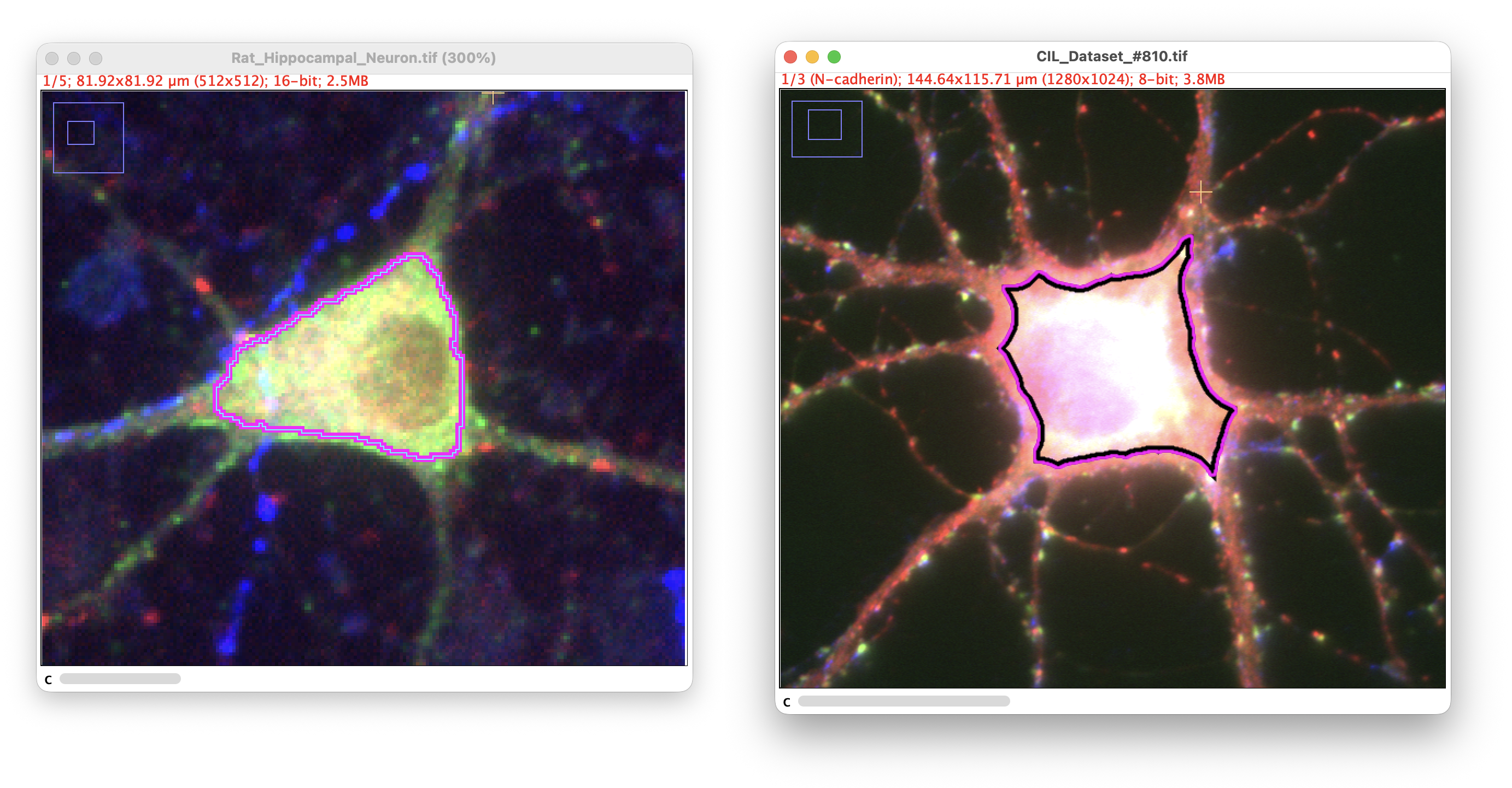
Automated soma detection: ROI countour (Cultured hippocampal neurons: Neuronal receptors/Synaptic labeling demo datasets)
Detection Strategy
The algorithm uses a combined EDT-intensity approach to identify somas:
- Euclidean Distance Transform (EDT) identifies the thickest structures in the image. Since somas are typically the thickest part of neurons, they have the highest EDT values
- Intensity scoring weights the EDT by pixel intensity to favor bright structures
- The product of EDT × intensity identifies regions that are both thick and bright, typical characteristics of well-labeled cell bodies
This dual approach is more robust than using intensity alone because it effectively filters out hot pixels and imaging artifacts, which are bright but thin (low EDT values).
Detection Scope
Brightest/largest soma only Detects the single most prominent soma in the image—the structure with the highest EDT × intensity score. Use this for images containing a single neuron or when you want to identify the primary cell body.
All somata in image Detects multiple somas by finding local maxima in the EDT map. Each local maximum represents a thick structure that likely corresponds to a cell body. When this scope is selected, several additional filtering parameters become available (see below).
Threshold
The intensity threshold determines which pixels are considered foreground during detection. Use -1 (default) to automatically compute the threshold using image statistics. Manual adjustment may be needed for images with uneven illumination or weak signal.
Multi-soma Filtering Parameters
The following parameters are only active when the detection scope is set to All somata in image:
Min. radius The minimum soma radius in spatially calibrated units. Detections with an EDT-derived radius below this value are discarded as noise (debris, hot pixels, etc.). Default: 0 (no filtering).
Min. inter-soma distance The minimum distance between detected soma centers in spatially calibrated units. When greater than zero, non-maximum suppression is applied: among detections that are closer than this distance, only the one with the highest EDT × intensity score is kept. This is the most reliable way to separate closely spaced detections. Default: 0 (disabled).
Expected no. of somata [Experimental] When greater than zero, keeps only the top-N detections ranked by EDT thickness. This uses an additional binarization step (Minimum auto-threshold) to recompute the EDT and rank candidates, which may not work well for images with large connected bright regions. In most cases, Min. inter-soma distance (above) is a more reliable filtering strategy. Default: 0 (disabled).
Output Types
Results can be exported in several formats. When detecting all somata, the output is added to the image overlay (for ROI types) or to the Path Manager (for path output):
-
Single-node path Creates a path in SNT’s Path Manager consisting of a single node at the soma center. The node radius is estimated from the distance transform. Useful for marking soma locations in reconstructions and for seeding multi-soma autotracing
-
Point ROI Places a point marker at the detected soma center. Simplest output for marking locations
-
Area ROI Creates a contour ROI outlining the soma boundary, determined by flood-filling from the center at the detection threshold. Useful for measuring soma size or creating exclusion regions
-
Circular ROI Draws a circle centered on the soma with radius estimated from the distance transform. Approximates soma size when the cell body is roughly spherical
Multiple Cells
The Auto-trace › Grayscale Image (Multiple Cells)… command traces all cells in a grayscale image in a single run. It automatically detects all soma locations, then traces each cell independently using the GWDT + Fast Marching pipeline with exclusion masks that prevent territory overlap between cells.
")
The command shares the same tracing parameters as the single-cell variant (thresholding, branch filtering, scoring, post-processing, smoothing, and resampling) but replaces the Soma/Root Detection section with parameters specific to multi-cell reconstruction.
Accurate soma detection is essential for multiple-cell autotracing. The multi-soma pipeline traces each cell independently from its detected soma, so any missed or spurious detection will propagate through the entire reconstruction. Strategies for ensuring the correct cell count can be further tuned using scripting.
This approach assumes spatially separable cells. Because each traced voxel is exclusively assigned to the nearest soma via the exclusion mask, arbors that intertwine in the same territory will be truncated at the boundary claimed by the first-traced cell. For dense neuropil with overlapping arbors, instance segmentation (e.g., deep-learning-based voxel classification) or spectral separation (e.g., multicolor labeling) would be needed to disambiguate cells prior to tracing.
Soma Detection
These are the filtering parameters for soma detection described earlier.
Territory Control
Territory reach Controls how far each cell’s tracing can extend toward its nearest neighbor, expressed as a fraction of the inter-soma distance. At 0.5 (default), each cell traces up to the midpoint between somas, so territories just touch. Values above 0.5 allow territories to overlap—the exclusion mask still prevents actual re-tracing. Set to -1 to disable territory limits (unlimited spread)
Multi-Cell Options
Exclusion buffer (voxels) After tracing from one soma, the traced voxels are dilated by this buffer before being masked out in subsequent Fast Marching runs. Larger values create wider exclusion zones, preventing re-tracing of neurites already claimed by another cell. Default: 5 (set to 0 to disable)
Min. paths per cell Minimum number of paths a traced cell must have to be retained. Cells producing fewer paths (e.g., soma-only traces with no neurites) are discarded. Default: 2
A batch variant is available under Auto-trace › Batch Processing for processing directories of images. Each image is processed independently with automatic soma detection, and results are exported as SWC files (one per detected cell).
Scripting
Fully automated tracing of multiple cells in a single image is also supported via scripting.
Accurate soma detection is essential for multiple-cell autotracing. Strategies for ensuring the correct cell count, from least to most accurate:
- Fully automatic detection with defaults:
SomaUtils.detectAllSomas()with default parameters. Convenient but sensitive to image quality and cell density - Tuned filtering parameters: Adjusting Min. radius and Min. inter-soma distance to match the expected cell morphology (see Multi-soma Filtering Parameters)
- Expected number of somata: Setting the expected count to keep only the top-N candidates ranked by EDT thickness. Experimental; may not work well for images with large connected bright regions
- User-provided coordinates or ROIs: Supplying exact soma locations via
SomaUtils.detectSomasAt(). The most reliable approach: bypasses all heuristic detection, giving you full control over which cells are traced. When using curated seeds, callsetAutoFilter(false)on the tracer to prevent heuristic filtering from discarding valid somas
The general workflow is:
- Detect soma locations: Either automatically using
SomaUtils.detectAllSomas(), or from user-provided seed coordinates / ROIs usingSomaUtils.detectSomasAt() - Configure the tracer: Set up a GWDT tracer with appropriate parameters. When using user-provided seeds (from ROIs or manual coordinates), call
setAutoFilter(false)on the tracer to prevent heuristic filtering from discarding valid somas - Trace: Pass the detected somas to
traceMultiSoma(), which runs the full GWDT + Fast Marching pipeline independently for each soma, with exclusion masks preventing traced territories from being retraced
Here is a minimal Groovy example using ROI-based seeds:
#@ SNTService sntService
import sc.fiji.snt.tracing.auto.GWDTTracer
import sc.fiji.snt.tracing.auto.SomaUtils

// Assumes SNT is running with an image loaded and ROIs marking soma locations
def snt = sntService.getInstance()
def imp = snt.getImagePlus()
def rois = imp.getOverlay().toArray() as List

// Detect somas at ROI centroids:
//   imp  - the ImagePlus with the image data
//   rois - collection of ROIs whose centroids mark soma locations.
//          Z is derived per ROI from Roi.getZPosition(); ROIs not
//          associated with a slice have Z resolved via MIP-based lookup
def somas = SomaUtils.detectSomasAt(imp, rois)

// Initialize the GWDT tracer:
//   1st arg - the image as an ImgPlus (false = do not duplicate)
//   2nd arg - background threshold (-1 = auto-estimate via Otsu)
def tracer = new GWDTTracer(snt.getLoadedDataAsImg(false), -1)
tracer.setAutoFilter(false) // disable heuristic filtering: seeds are user-curated

// Trace all cells and add results to the Path Manager
def trees = tracer.traceMultiSoma(somas)
println("Traced ${trees.size()} cell(s)")
sntService.addTrees(trees)
For automatic seed detection (no ROIs required), replace the seed detection step with:
def img = snt.getLoadedDataAsImg(false) // get loaded data as ImgPlus
// detectAllSomas parameters:
//   img        - the image as an ImgPlus
//   threshold  - intensity threshold (-1 = auto via Otsu)
//   zSlice     - Z-slice (0-indexed; -1 = auto: per-soma auto detection using MIP-based intensity lookup)
//   minRadius  - minimum soma radius in pixels (filters out small detections)
//   minDist    - minimum inter-soma distance in pixels (0 = no NMS filtering)
def somas = SomaUtils.detectAllSomas(img, -1, -1, 10, 0)
Look for the AutoTracing_Demo(Microglia_Cells)_ demo script for other details.
Segmented Images
Segmented (binary or thresholded) images are processed using skeleton-based tracing, which converts the image topology into neuronal tree structures. This approach is suitable for images with clear foreground/background separation where structures have already been segmented through thresholding or other preprocessing methods.
The algorithm works by first skeletonizing the segmented image to extract its topological structure, then converting the resulting skeleton graph into neuronal trees. Segmented images are processed using the Auto-trace › Segmented Image… command when the image to be processed is already open or Auto-trace › Segmented Image File…, if the image is yet to be loaded from disk. For technical implementation details including the skeletonization algorithm and graph conversion methods, see the SNT technical notes.
You can follow these instructions using File › Load Demo Dataset… and choosing the Drosophila ddaC neuron (Autotrace demo). It will load a binary (thresholded) image of a Drosophila space-filling neuron (ddaC) displaying autotracing options for automated reconstruction.
Input Image(s)
Full automated tracing of segmented (thresholded) images requires two types of inputs:
-
Segmented Image (Mandatory) The pre-processed image from which paths will be extracted. It will be skeletonized by the extraction algorithm. If thresholded (recommended), only highlighted pixels are considered, otherwise all non-zero intensities in the image will be considered for extraction.
-
Intensity Image (Optional) The original (un-processed) image used to resolve any possible loops in the segmented image using brightness criteria. Required for intensity-based loop resolution strategies (see below).
")
Soma/Root Detection
Root detection typically uses an area ROI to mark the root of the arbor on the image. With neurons, this typically corresponds to an area ROI marking the soma. Several strategies are possible:
-
Place root on ROI’s simple centroid Attempts to root all primary paths intersecting the ROI at its geometric centroid (the centroid of the ROI’s contour). Typically used when 1) multiple paths branch out from the soma, 2) the ROI accurately defines the contour of the soma, and 3) somatic segments are expected to be part of the reconstruction
-
Place root on ROI’s weighted centroid Similar to the above, but places the root at the centroid of all foreground voxels contained by the ROI, rather than the ROI’s geometric center. Useful when the ROI contour is imprecise but still encloses the relevant structure
-
Place roots along ROI’s edge Attempts to root all primary paths intersecting along the perimeter of the ROI. As above, this option is typically used when multiple paths branch out from the soma and the ROI defines the contour of the soma, but somatic segments are not expected to be included in the reconstruction. Most accurate strategy for complex topologies
-
ROI marks a single root Assumes a polarized morphology (e.g., apical dendrites of a pyramidal neuron), in which the arbor being reconstructed has a single primary branch at the root. Under this option, the ‘closest’ end-point (or junction point) contained by the ROI becomes the root node. In this case the ROI does not need to reflect an accurate contour of the soma
-
None. Ignore any ROIs If no ROI exists an arbitrary root node is used
When parsing 3D images, toggling the Active plane only checkbox clarifies that the root(s) marked by the ROI occurs at the active ROI’s Z-plane. This ensures that other possible roots above or below the ROI will not be considered.
Loop Resolution
Skeletonized images often contain spurious loops (cycles) that must be broken to produce valid tree structures. Several strategies are available:
-
Dimmest branch Removes the branch with the lowest average intensity in the loop. Requires an intensity image. Best when signal intensity correlates with structural importance
-
Dimmest voxel Cuts the loop at the single dimmest pixel. Requires an intensity image. More precise than dimmest branch but may be sensitive to noise
-
Shortest branch Removes the shortest branch (the skeletonized path between junctions) in the loop. Fast and suitable for simple artifacts, but may inadvertently break main structures
-
Shortest segment Removes the shortest edge(s) using a maximum spanning tree algorithm. Preserves the longest continuous paths in the structure. Suitable for simple loops where geometric length indicates “importance”
-
Furthest from root Removes edges most distant from the root/soma. Preserves proximal structure closer to the cell body. Requires a root-defining ROI. Only available when an ROI has been provided. Useful when loops near the soma are expected to be more meaningful/important than distal ones
-
Peripheral segments Removes edges with the lowest betweenness centrality (i.e., edges that lie on fewer shortest paths through the graph). Preserves the main backbone/trunk of the structure regardless of geometric length. Recommended for complex structures where topological importance matters more than geometry
NB: If an intensity-based strategy is selected but no intensity image is provided, the algorithm automatically falls back to Peripheral segments.
Gaps and Disconnected Components
It is almost impossible to segment structures into a single, coherent volume. These options define how gaps in the segmentation should be handled.
-
Settings for handling small components These options determine whether the algorithm should ignore segments (connected components that are disconnected from the main structure) that are too small to be of interest. Disconnected segments with a cable length below the specified length threshold will be discarded by the algorithm.
Increase this value if too many isolated branches are being created. Decrease it to bias the extraction for larger, contiguous structures. -
Settings for handling adjacent components If the segmented image is fragmented into multiple components (e.g., due to ‘beaded’ labeling): Should the algorithm attempt to connect nearby components? If so, what should be the maximum allowable distance between disconnected components to be merged?
You should increase Max. connection distance if the algorithm produces too many gaps. Decrease it to minimize spurious connections.
NB: When components are bridged, new loops may be introduced. These are automatically resolved using the selected loop resolution strategy.
Use Path Orientation (hold O) to verify path orientations. Hold F to temporarily hide all annotations.
Additional Options
Additional processing options are available in the dialog:
Prune single-node paths Whether single-point paths without children should be filtered out from the final reconstruction.
After tracing As described earlier, this option determines what happens after the traced trees are added to the Path Manager.
Batch Processing
All autotracing commands (grayscale single-cell, grayscale multi-cell, and segmented image) can process entire directories of images in batch mode. Batch commands are available from the Auto-trace menu under the Batch Processing separator, or through the File › Load Tracings import menu.
In batch mode, all tracing parameters are configured once and applied uniformly to every image in the input directory. Each image is loaded, traced, and the resulting reconstruction is exported as an SWC file to the specified export directory. For multi-cell batch processing, each detected cell produces a separate SWC file (named <image>_cell1.swc, <image>_cell2.swc, etc.). Processing errors on individual images are logged but do not halt the batch, so the remaining images continue to be processed.
Batch Parameters
Path to image(s) The directory containing images to be traced or a path to a single file (e.g., an OME-ZARR, or .IMS file) that may be too large to fit into memory.
NB:
-
The Browse button may not allow you to select a folder directly: In that case simplify select a file within that folder, and manually remove it from the resulting path. E.g., if the goal is to parse
/path/to/folder/, browse to/path/to/folder/random.file, and delete “random.file” from the file path -
For grayscale tracing, images should contain bright neuronal structures on a dark background. For segmented image tracing, images should be binary masks or thresholded images where non-zero pixels represent foreground structures.
Export directory The output directory where SWC files will be saved. One SWC file is generated per input image.
All other tracing parameters (thresholds, filtering, post-processing, etc.) are shared with the corresponding interactive command and apply to every image in the batch. Soma/root detection defaults to automatic in batch mode (no ROI interaction).