What is colocalization?
Suppose you are given some images by a colleague, or have some images of your own, and you want to measure the amount of colocalisation between two of the dyes or stains in the images. First you have to define what you mean by colocalisation, and that is not trivial. Generally speaking, when we evaluate colocalization, we are usually attempting to demonstrate that a significant, non-random spatial correlation exists between two channels of a dual color image. The specific nature of that correlation, and what it means for your research, can vary quite a bit. It could mean that one signal of one channel is contained within the bounds of another, or that your stains/dyes are typically found separated by a certain distance or are generally clustered, or simply that the signal from both channels overlap each other when imaged at a particular spatial resolution. Importantly, colocalization results cannot indicate that two proteins/molecules are bound or interacting, only that they are both localized to within a certain volume, and is mostly dependent upon your microscope and its acquisition parameters. Regardless of your microscope, this volume is many, many times greater than the volume of a single protein. For this reason, colocalization is most often used to determine if a protein is localizing to an organelle or other well defined cellular structure.
For more information on colocalisation and for how to correctly capture quantitative fluorescence microscopy images suitable for colocalisation analysis, look here: Image Processing Courses at BioDIP, Dresden. A recent review is by Dunn in 2011.
State the resolution explicitly!
The Pauli exclusion principle states that two particles cannot have the same quantum numbers so they cannot be in the same place. So, actually nothing is “really” colocalised. At the other extreme, a universe of one voxel (not cubic of course) is completely colocalised - everything is inside it. Practically, our situation lies between the two extremes. We must colocalise at some defined and explicit spatial scale: In our case the optical resolution or image pixel/voxel spacing, whichever is the larger value in nm, micrometers, mm, meters, km, etc. The colocalization measurement we make only means anything in relation to the spatial scale we are working at, so it needs to be explicitly stated. Additionally, the spatial resolution of your image must be sufficient to actually support your hypothesis. You can find more details about optical resolution and image pixel spacing in the “Notes and precautions” section below.
“Color” doesn’t matter
In the majority of fluorescence microscopy images, all the “colors” of a multi-channel image are captured using a monochromatic detector that doesn’t know what color the photons that hit it are; that is determined by the fluorescence emission filters we use. Hence, any colors displayed are false. These false colors are only useful to tell which channel is which. If I want to show DAPI in green and EGFP as magenta, there is nothing “wrong” about that.
When considering colocalization, too often composite images of red and green channels are considered sufficient. This is plain wrong. The problems with red/green merge images, aside from obvious issues with red-green colour-blind people, is that the perception of human eyes and brain can be fooled very easily. Just have a look at this image:
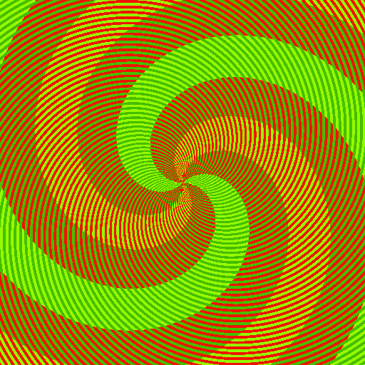
Most people might think that the image contains 4 distinct colours: 2 sets of thin spirals are in dark red and dark green, and 2 thick prominent spirals of yellow-green and yellow. However, the yellow and yellow-green actually have exactly the same color! You can verify this yourself by calling File › Open Samples › Spirals Macro in Fiji.
So… now, how do you feel about determining colocalization by looking for yellow blobs? Doesn’t make much sense does it? We notice that the shades and hues of colours look different according to what other colours they are next to! So, you need to measure something from the pixel values, not simply subjectively “look at” a red/green colour merge image.
An even better reason to always quantitatively evaluate colocalization is that this actually tells you what you are looking for - the correlation (or not) between 2 channels of pixels over space.
Methods of colocalization analysis
As there are many different reasons you may perform a colocalization analysis when evaluating your images, and many different microscopy techniques you could have used to acquire those images, there are also many different methods of evaluating colocalization. There is no universal best method, each has its own advantages and disadvantages, but some methods may be better suited for your data or hypothesis.
Pixel intensity-based
In intensity-based correlation analyses, the pixel/voxel values in the image are directly used in the evaluation of spatial correlation. These can be broadly divided into two types: pixel matching colocalization analyses, and cross-correlation function based analyses.
Pixel-wise methods
In pixel-wise colocalization analyses, the intensity of a pixel in one channel is evaluated against the corresponding pixel in the second channel of a dual-color image, generally producing a scatterplot from which a correlation coefficient is determined. As these methods are straightforward, work very well with traditional widefield fluorescence imaging, and are very well founded as some of the earliest methods for measuring colocalization, they are very widely used. However, the pixel-wise matching means that there must be overlap of the signal from the two channels to demonstrate positive spatial correlation. This can be problematic for super-resolution microscopy images, where the improved resolution means that even close, strongly-correlated proteins may not produce sufficient overlap after imaging to work with these colocalization methods. Additionally, it is critical that the spatial resolution is reported when using this method, as the scale and resolution of the image can affect the results and their interpretation!
Here are just two of many colocalization coefficients to express the intensity correlation of pixel-wise colocalizing objects in each component of a dual-color image:
- Pearson’s correlation coefficient. It is not sensitive to differences in mean signal intensities or range, or a zero offset between the two components. The result is +1 for perfect correlation, 0 for no correlation, and -1 for perfect anti-correlation. Noise makes the value closer to 0 than it should be.
- Manders split coefficients. Proportional to the amount of fluorescence of the colocalizing pixels or voxels in each colour channel. You can get more details in Manders et al. Values range from 0 to 1, expressing the fraction of intensity in a channel that is located in pixels where there is above zero (or threshold) intensity in the other colour channel.
These coefficients measure the amount or degree of colocalization, or rather correlation and co-occurrence respectively (but should not be expressed as % values, because that is not how they are defined). But if there is nothing to compare them to, what do they mean? A statistical significance test was derived by Costses to evaluate the probability that the measured value of Pearson’s correlation r between the two colour channels is significantly greater than values of r that would be calculated if there was only random overlap of the same information. This test is performed by randomly scrambling the blocks of pixels (instead of individual pixels, because each pixel’s intensity is correlated with its neighboring pixels) in one image, and then measuring the correlation of this image with the other (unscrambled) image. You can get more details in Costes et al. The result of this tests tell us if the Pearsons r and split Manders’ coefficients we measure are better than pure chance or not.
The example below (Thanks Tony Collins for this nice figure), generally demonstrates the type of results generated by pixel-wise colocalization analyses.
 Channel 1
 Channel 2
 Coloc Scatterplot
 Scatterplot with Quadrants
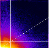
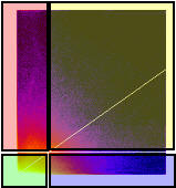
In the scatterplot or 2D Histogram the two intensity values for each pixel or voxel are plotted against each other, and the brighter the colour, the more pixels or voxels have those two intensity values for their two colour channels. Here we see if there is correlation immediately by eye, in the presence of a cloud of information in the middle of the 2D histogram. We can fit that cloud with a linear regression and measure correlation coefficients. After setting thresholds in both colour channels, we see the scatterplot or 2D Histogram is split into 4 areas, quadrants. The contents of each can be used to calculate different colcoalization results.
Other coefficients include ranked correlations such as Spearman and Kendal’s Tau, and Li’s ICQ. Some others are described in the literature, but that have been refuted as insensitive, such as the overlap coefficient from the Manders paper, which J. Adler et al. showed to have large problems in interpretation compared to Pearson’s r and Manders’ split coefficients.
Cross-correlation function
Another type of intensity-based colocalization analyses utilize the Cross-correlation (CCF) to evaluate correlation between two channels. Exploring these techniques in the literature can be very confusing as there are effectively two different ways to apply the cross-correlation function to the problem of colocalization, and the distinction between them is often not well delineated in manuscripts discussing these techniques, with no consistent naming convention distinguishing one from the other. The two different ways that the CCF can be evaluated are either as a function of distance (spatial cross-correlation) or time (temporal cross-correlation). While these both use the same root function, they are two very different methodologies that have different imaging requirements, and that provide very different information about your molecules/proteins.
Spatial cross-correlation
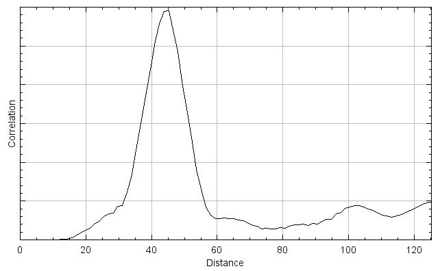
In spatial cross-correlation, initially a measure of correlation of the two channels of a dual color image are evaluated in a manner similar to the pixel matching methods described above (though the exact function may vary). Then, one channel is shifted relative to the other (typically by one pixel) and then correlation is re-evaluated with that offset. This process is repeated across the entire image to generate a curve of correlation as a function of distance, as shown to the right. Like the scatterplot generating methods above, spatial cross-correlation methods work on single images and do not require more than one time point.
A key advantage of this method type is that the fluorescent signal from the two channels does not need to overlap to demonstrate spatial correlation, which also makes these methods more compatible with super-resolution imaging. Additionally, any resolution or signal density limits in the image are captured in the curve generated by the function, since this curve is a function of distance. Thus, as long as the curve is adequately described in the results (by standard deviation of a Gaussian fit or FWHM) the spatial resolution of the microscope would not need to be reported. However, image cross-correlation can be very computationally intensive compared to the one to one pixel matching methods, since the correlation needs to be evaluated after every image shift. This can be sped up by limiting the distance and/or axis over which the correlation is evaluated, or by performing the cross-correlation calculation in the frequency domain, but these methods are still typically slower than the methods described above.
Temporal cross-correlation
In temporal cross-correlation two stained molecules are simultaneously monitored over time for coincident fluctuations in intensity. Coincidence of the fluorescence intensity fluctuations generally indicates molecular interaction. The key difference in temporal cross-correlation when compared to spatial cross-correlation, is that with temporal cross-correlation the data is shifted through time, not through space. Thus, any temporal cross-correlation technique will require acquisition over time, and cannot be performed on single frame images or fixed samples.
The first, and best known, temporal cross-correlation technique is Fluorescence cross-correlation spectroscopy (FCCS). In FCCS a single diffraction limited volume is illuminated with two excitation lasers using a confocal microscope, and the emission of two fluorophores is recorded simultaneously over time. The two resulting fluorescent fluctuation graphs are then cross-correlated to determine if the particles are moving together, indicating an interaction. However, this technique does not need to be limited to a single focal volume, and more recent implementations of temporal cross-correlation apply this same methodology to multi-frame images, effectively evaluating the FCCS at each pixel of the image and averaging it. These image based temporal cross-correlation implementations are usually referred to as image cross-correlation spectroscopy (ICCS), however, this term has also been applied to spatial cross-correlation methods, which can make it very difficult to find the appropriate technique. If you’re ever unsure, the graphs generated from temporal cross-correlation methods will have their x-axis as time (usually labeled as τ or seconds), and not pixels or microns.
Object-based colocalization
In object-based colocalization analyses, the image is first segmented to separate the objects of interest from the background for both channels. Colocalization is then evaluated using these binary images, generally by comparing the area/volume of the intersection of the two images to the area/volume of: a) the union of the binary images, b) the difference of the binary images, c) one of the binary images unaltered, or d) a combination of these three. What you compare the intersection against will depend on the exact question being asked. Being able to tailor the analysis to your specific circumstances is one of the biggest advantages to object based-analysis. Additionally, basic object-based analyses can be performed easily without use of a plugin (though some are available to streamline the process) by doing the following: After segmentation of both images, the Image Calculator (Process › Image Calculator…) can be used to generate the intersection (AND operator), difference (difference or subtract operator), and the union (add or OR operator). Once these have been created, they can be analyzed using particle analysis to determine the area/volume, or analysis can be redirected to the original intensity data (Analyze › Set Measurements…) to evaluate the original pixel density within the particles. Generally, this type of object-based colocalization does require that there is overlap between your objects of interest from each channel. However, plugins have been developed that will perform distance analysis on the original binary images, removing the requirement for overlap between the two channels.
SMLM colocalization
Due to the unique nature of single-molecule localization microscopy images, as a list of localized points rather than a matrix of intensity values, traditional intensity or object-based colocalization techniques are insufficient for their analysis and thus SMLM images have their own unique colocalization methods. There are presently two categories of SMLM colocalization methods, neighboring colocalization and Voronoï-based colcoalization anlaysis.
Plugins for colocalization
There are several plugins available for performing colocalization analysis. In addition to the options described below, see also the list of extensions Colocalization category.
List of plugins by method type
- One to one pixel matching analyses:
- Coloc2
- JaCoP
- Colocalization finder
- Colocalization Threshold (deprecated)
- Colocalization Test (deprecated)
- Spatial cross-correlation analyses:
- Temporal cross-correlation analyses:
- Object-based analyses:
- SMLM analyses (no ImageJ implementations):
- Coloc-Tesseler (standalone, not an ImageJ plugin)
- ClusDoC (MatLab plugin)
Details on popular ImageJ colocalization plugins
Coloc 2
Coloc 2 implements and performs the pixel intensity correlation over space methods of Pearson, Manders, Costes, Li and more, for scatterplots, analysis, automatic thresholding and statistical significance testing.
None of this gives sensible results unless you have your imaging hardware set up appropriately and have acquired images properly, and have performed appropriate controls for bleed-through and chromatic shift etc. See here for hardware set up guidelines.
This plugin supersedes the Colocalization Threshold and Colocalization Test plugins, which unfortunately were buggy and hard to maintain. So we started from scratch with a carefully planned and designed new plugin. While the old plugins are described below as well, we recommend that you use Coloc 2 instead.
One main feature of Coloc 2 is the standardised PDF output, which is intended to make the results of different colocalization experiments comparable.
Please see the Coloc2 page for complete instructions on using the Coloc 2 plugin, including common pitfalls of the pixel intensity spatial correlation methods that it employs.
JaCoP
JaCoP is a compilation of co-localization tools:
- Calculating a set of commonly used co-localization indicators:
- Pearson’s coefficient
- Overlap coefficient
- k1 & k2 coefficients
- Manders’ coefficient
- Generating commonly used visualizations:
- Cytofluorogram
- Having access to more recently published methods:
- Costes’ automatic threshold
- Li’s ICA
- Costes’ randomization
- Objects based methods (2 methods: distances between centers and center-particle coincidence)
All methods are implemented to work on 3D datasets.
See the JaCoP page for full details.
Colocalization Finder
The Colocalization Finder plugin displays a correlation diagram (called scatterPlot picture) from two initial pictures having the same size together with a RGB overlap of the original images (called Composite picture).
See the Colocalization Finder web page for further details.
Sample datasets
This first sample data set that has very good colocalization because the 2 subunits of a dimeric protein are stained with green and red dyes respectively. The methods of Pearson, Manders, Costes and Li should work very well for this sample, but this dataset fails many of the quality checks addressed in the section below.
colocsample1bRGB_BG.tif: Use the “Image > Color > Split Channels” menu command to get a separate z stack for the 2 dyes (you can throw the blue one away!).
In addition to this dataset, Fiji comes pre-loaded with many sample images found under the “File > Open Samples” menu. Of these, there are a few multi-channel images that can be used as inputs in Colocalization plugins (though they don’t necessarily have any spatial correlation between the channels):
- Confocal series
- Fluorescent Cells
- Fly Brain
- HeLa Cells
- Mitosis (multi-frame image)
- Neuron (good colcoalization between red and green channel)
- Organ of corti
- First instar brain
Notes and precautions
2D or 3D images?
Cells, and everything within them and outside of them, exist and relate to one another in 3 spatial dimensions. Whenever possible you should perform 3D colocalization analyses. You can even evaluate 3D colocalization over time in living cells/systems (4D colocalization anlaysis) for even more comprehensive results.
Check your image quality!
Questions you should ask before attempting colocalisation analysis from 2 colour channel images:
- Is the image data noisy?
- Has there been lossy compression?
- Is the intensity information saturated / clipped / overexposed?
- Is there a problem with uniform background / detector offset?
- What is the spatial resolution and is it sufficient to support my hypothesis?
To begin with, we should check the images for problems that might make the colocalisation analysis methods fail or be unreliable.
- Significant noise (uncertainty in the pixel values - usually from detection of too few photons) means the methods we will use will significantly underestimate the true colocalization, or even completely fail to give the true result.
- Lossy compression messes up the intensity information of the pixels, causing the colocalization result to be more or less wrong.
- Intensity clipping/saturation is bad news. Pixel intensity correlation measurements rely on the pixel intensities being true and not clipped to 255 when they were really higher! See the Detect Information Loss tutorial for details on how to detect such problems.
- We should look for wrong offset / high background (since this confuses the auto threshold method, since zero signal is not zero pixel intensity but some larger number)
- Spatial resolution:
The spatial resolution of the images, by definition, determines the spatial resolution that you are measuring colocalization at. The results will be different at different levels of spatial resolution. If the image is one big pixel, everything will colocalize!
The spatial resolution of the light microscope is limited by the wavelength of the light (and the NA of the objective lens) according to Ernst Abbe’s work. Molecules / proteins are an order of magnitude smaller than the wavelength of visible light, so they could be many nm apart, but still appear in the same image pixel. Is that true colocalization? Maybe, but it depends how you define it!
Are the images spatially calibrated? If not then we need to calibrate them so we know the spatial sampling rate (think pixel or voxel size) in x, y and z. See the SpatialCalibration tutorial for how to do that. We need the images to be spatially calibrated in order for the Costes statistical significance test (below) method to work properly.
We need to think carefully about the correct or adequate spatial resolution in x, y and probably z. This depends on the Numerical Aperture of the objective lens. You can calculate the correct pixel or voxel sizes for the objective lens you are using, to get the maximum resolution that that objective lens can really see: [Nyquist Calculator](https://svi.nl/NyquistCalculator]. Essentially the pixels / voxels should be about 3 times smaller than the resolution of the lens. On the other hand, if you are only interested in larger objects, and not the smallest details the objective can see, it makes sense to have larger pixels or voxels. Again, these should be about 3 times smaller than the smallest feature you want to resolve.
Nyqvist tells us the spatial sampling should be about three times smaller than the smallest object we want to resolve. Remember, spatial intensity correlation analysis, as we will perform here, cannot tell you that 2 proteins are bound together in some biophysical bonding interaction. However, it might suggest that the 2 molecules occur with the same relative amounts when they are present in the set of spatial samples (pixels or voxels) with intensities above the thresholds we will calculate below. In any case, it might be a hint that “maybe they are binding partners or in the same macromolecular complex”. You should follow up by determining true binding using FLIM, FRET and biochemical methods like Immuno co-Precipitation etc.
Further reading
- Image co-localization – co-occurrence versus correlation.
- A practical guide to evaluating colocalization in biological microscopy.
Older colocalization plugins
Colocalization Threshold
Note: this plugin is no longer under active development and support. Use Coloc 2 instead, which does the same thing, only better.
The Colocalization Threshold plugin performs several functions for you in one go. With the “green” and “red” stacks of the colocsample1bRGB_BG.tif dataset open and the channels split (see above) choose the menu item “Analyze-Colocalization-Colocalization Threshold”. Next select the right stacks for the analysis in Channel1 and Channel2. You can use a region of interest (ROI) if you like, which should be defined before you run the plugin. Check on “Show Colocalized Pixels” and “Show Scatter Plot” (see also Why scatter plots?), and others off. You can explore the options in Set options. Turn ALL the options on the first time you use it, so you see what it can do.
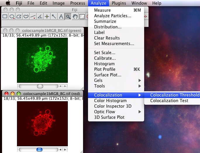 Opening the plugin
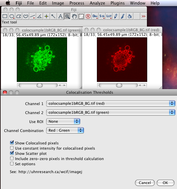 Options
 Output
- It generates a 2D Histogram / Scatterplot / Fluorogram. this is a really good way to visualise the correlation of the pixel intensities, over all pixels/voxels in the image, and can tell you immediately about problems such as intensity saturation/clipping, wrong offset, emission bleedthrough (fluorescence signal from the wrong dye in the detection channel), and even if there are multiple populations of colocalising species with different ratios of dyes in the same sample. Think of it just like a FACS or Flow cytometry scatter plot; indeed it is very similar.
- It makes a linear regression fit of the data in the scatter plot. That is the diagonal white line in the scatter plot, the gradient of which is the ratio of the intensities of the 2 channels.
- It does the Costes method auto threshold determination. The thresholds are the intensity levels above which for both channels you say the two dyes are “colocalised”. This method uses an iterative procedure to determine what pair of thresholds for the 2 channels of the scatterplot give a Pearson’s correlation coefficient (r) of zero for the pixels below the thresholds. That means that all the pixels which have intensities above the two thresholds have greater than zero correlation, and the pixels below the thresholds have none or anti correlated intensities. The method is pretty robust (so long as you don’t stupidly defeat it, i.e. with image data with high offsets / background), and is fully reproducible, meaning you will always get the same thresholds for the same data set, and similar thresholds for similar datasets. Threshold setting is a big problem in colocalisation analysis. If you use a tool that allows you to manually set the thresholds, obviously you can get any result you like, since you are subjectively deciding what is colocalised and what isn’t. This might please your boss, but it’s not very scientific is it? So don’t do that! Use the Costes auto threshold instead! Some people say the Costes method sets the thresholds too low, and lower than they would set them by eye. That might be true, but manual methods are subjective and totally unreliable. The thresholds that Costes method sets always mean the correlation below the thresholds is zero. That’s a good thing.
The plugin finally sends a bunch of statistics and results to the results window. You need to turn them all on using the “set options” checkbox of the plugin GUI. Some of these results are pretty uninformative. They are listed here, in arguably order of usefulness:
- The thresholded Mander’s split colocalisation coefficients (zero is no colocalisation, one means perfect colocalisation. There is one coefficient per channel, which tells you the proportion of signal in that channels that colocalises with the other channel. Of course this might be different for the two channels! The thresholded Mander’s coefficients are probably the numbers you would publish (not the Pearson’s coefficients as these are less informative).
- The thresholds that were set by the Costes Auto threshold method.
- The Pearson’s coefficients for: the whole image, image above thresholds (should be close to 1 for very good colocalizing dyes) and image below thresholds (should be around zero, because that’s how the Costes auto threshold method tries to set them… so if it is not close to zero, something went wrong!)
- Linear regression solution: If the image data are close to ideal, with comparable mean intensity in both channels and no problems exist with offset/background, then by definition, the gradient of the regression line will be close to unity (1) and the intercept will be close to zero. These are both good things for the quality of the result. This information might be less useful in other situations, e.g. where there is only sparse data in one channel, or there are multiple colocalising populations of signals (several clearly independent patches/blobs in the scatterplot).
- The % volume and intensity colocalised values are pretty useless, unless you use a biologically relevant region of interest, as they are very dependent on how much stuff and how much background there is in a certain image, and you will get totally different values for different images of the same sample, that happen to have different areas of background. In images that have no empty regions, like tissue samples, it might then be a useful number. Maybe % intensity above threshold colocalised might be a useful value in some cases? See section 6.3 at http://www.uhnresearch.ca/facilities/wcif/imagej/colour_analysis.htm for more explanation of what the different measurements exactly are, or look at the code.
Colocalization Test
Note: this plugin is no longer under active development and support. Use Coloc 2 instead, which does the same thing, only more correctly, and as described in the original publication by Costes, instead of making a nasty assumption and shortcut.
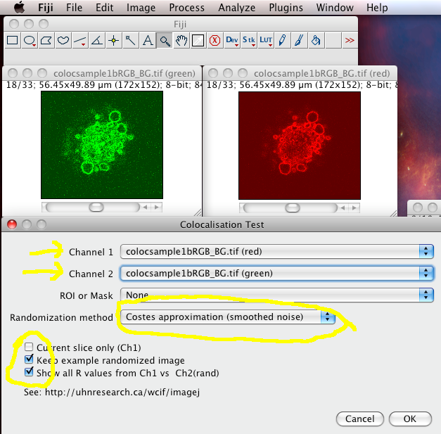
The Colocalization Test plugin performs the Costes test for statistical significance (which you should ALWAYS do after calculating the thresholded Manders coefficients and the scatterplot). It is in the menus at Analyze › Colocalization › Colocalization Test
Choose the correct Channel 1 and Channel 2 images stacks from the drop down lists. Make sure “Current Slice Only” is off, and “Keep Example Randomized Image” and Show All R values” are on. Then click “OK”
The results window will then display the calculated P-value, and some other details of the test calculation.
 Costes test configuration
 PSF details
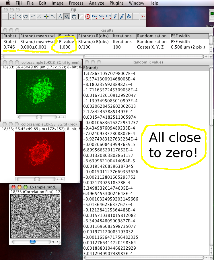 Result
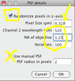
The Costes method for Statistical Significance relies on the spatial calibration of the image, knowledge of the Numerical Aperture (N.A.) of the objective lens, and the fluorescence emission wavelength to calculate how many pixels the point spread function covers in the image. Then it takes the image in one of the channels, and randomizes it by moving PSF sized chunks of the image to random locations in a new random test image. Then it calculates the Pearson’s correlation coefficient (r) between the randomized image and the original image of the other channel. If the correlation of the randomized image with the real image of the other channel is as good as or better than the correlation between the two real images, then any correlation that you measure is no better then what you would have got by chance for this image. This test is performed many (100) times, and the P-value is output, which is the proportion of random images that had better correlation than the real image. A P-value of 1.00 means that none of the randomised images had better correlation. 0.95 is the normal statistical confidence limit of 95%. Anything lower than that, and the correlation / colocalisation that you measure in the real images is not likely to be better than random chance, and thus is probably not interesting.
In this case the P-value should be 1.00. Since you told it to display the Pearson’s correlation (r) values (R values here), they are in another window. You can see they are all close to zero, and in the results you can see that on average the randomized R value is about zero, meaning that the randomized images all had no correlation with the real image. Which is a good thing!
Other available methods, such as Fay and Van Steensel, do the same thing but randomize the image in less rigorous but very simple ways, which may lead to errors such as over or under estimation of the P-value. However, they are faster than the Costes method.
Again, as for the Colocalization Threshold plugin, using an ROI here may well make very good sense, as you are only interested in the correlation between the 2 colour channels in parts of the image where the biology you are interested in is located. Background its typically uninteresting, and you can exclude it from the analysis. Its probably sensible to to use the same ROI as you used in the Colocalization Threshold plugin!