This page was last revised for version 5.1.0.
SNT integrates with deep-learning (DL) segmentation tools (e.g., cellpose, CSBDeep, DeepImageJ, nnU-Net, StarDist, and others) in both directions: their outputs — segmentations, probability maps, detected coordinates — become inputs to SNT’s tracing and analysis workflows, while SNT’s reconstructions, after curation and refinement, can be exported as ground-truth labels to train the next round of models. For simpler, classical-ML alternatives, SNT also embeds ensemble (random-forest) classifiers via Labkit/TWS. The sections below provide an overview of how model predictions can be consumed in SNT, and how SNT can be used to generate training data for either family of models.
Generating Training Data
SNT’s reconstruction, segmentation, and annotation tooling is also useful for producing training data for downstream models. The data SNT generates is well-suited as ground truth: it’s stored in calibrated coordinates, records provenance metadata, supports post-hoc refinements, and can be reviewed in the Curation Assistant before being used to train downstream models.
These aspects are covered elsewhere in the documentation:
-
Pixel-level labels for segmentation networks: Path Manager’s Process menu exports selected paths as classifier labels into Labkit/TWS. See Training Models below for the Weka-based workflow; the same exported labels can be repurposed for any U-Net-style trainer that consumes binary or multiclass images
-
Path fitting for automated refinement: The Refine/Fit command snaps each node onto the signal centerline and recomputes per-node radii from cross-sectional intensity profiles. The result is a geometry that hugs the actual neurite rather than the tracer’s first guess, lifting label quality before export
-
Editing tools for manual refinement: SNT’s Edit Mode (⇧ Shift + E) supports per-node manipulation: insert, delete, redirect, or paint stretches of a path directly on the image. Auto-traced or imported paths can be corrected to match the underlying signal precisely, producing higher-fidelity ground truth than a raw automatic trace would offer
-
Cross-over detections: The crossover detector flags places where neurites pass close together in 3D but aren’t topologically joined. Reviewing and resolving these before export prevents ambiguities from leaking into the training datasets
-
Curated reconstructions: Paths reviewed in the Curation Assistant can be exported (with their accept/reject status preserved in path tags) as either positive examples for training models that learn correct topology, or negative examples for QC-classifier training. A scriptable bridge between the Assistant and a training pipeline facilitates this, e.g.,:
import sc.fiji.snt.Tree
import sc.fiji.snt.analysis.curation.CurationTags
def tree = Tree.fromFile("/path/to/annotated/file.traces")
def p = CurationTags.partitionByReviewStatus(tree)
println "${p.positive().size()} +, ${p.negative().size()} -, ${p.unsure().size()} ?, ${p.unreviewed().size()}"
- Coordinate-only labels for detectors: the Seeded Tracing Assistant’s export commands write CSV files that any soma- or endpoint-detection model can ingest as positive examples. Manual annotations, ROI-derived seeds, and label-image-derived seeds can all be stored in the same exportable format
Embedded Tools: Labkit & TWS
SNT interacts with Labkit and Trainable Weka Segmentation (TWS), both leveraging machine learning algorithms for semantic segmentation of images (namely, random forest classifiers). The bridge between these tools makes it possible to:
- Import a pre-trained model into SNT and directly load the probability maps of the semantic segmentation as secondary tracing layer
- Train a model with SNT paths
The table below summarizes key differences between Labkit and TWS (as of SNT v5). Note that both tools classify images using the Weka framework.
| Labkit | TWS | |
|---|---|---|
| Image size | Out-of-core, multiple terabytes large image data | Smaller images (RAM-limited) |
| GPU support | via CLIJ2 | No |
| Underlying architecture(s) | ImgLib2 and BigDataViewer | ImageJ |
| Support for multichannel images | Yes | Yes (w/ caveats) |
| Support for timelapse images | Yes | Yes (w/ caveats) |
| Scripting and IJ macro language support | Yes. Some commands are macro-recordable | Yes. GUI is macro-recordable |
| Batch Processing | From GUI and via macros and scripts | Via macros and scripts |
| Import of pre-trained models into SNT | Yes | Yes |
| Direct loading of SNT paths as classification labels | Yes | Yes |
Importing Models
")
Importing of models can be done via the Secondary layer menu. Once the trained model is imported, it is applied to the image being traced, and the resulting classification is loaded as a secondary tracing image. The import prompt has the following options:
- Model file: The file to be imported. Typically, with a .model or .classifier extension (Labkit: JSON-encoded; TWS: XML-encoded)
- Loading engine: How the model should be loaded and applied. Either Labkit, Labkit w/ GPU acceleration or Trainable Weka Segmentation (TWS). NB: Labkit w/ GPU acceleration expects CLIJ2 access, and a CLIJ2-compatible graphics card
- Load as: Either Probability (p-map) or Segmented image. If Probability image, the class associated with neurite signal needs to be chosen in a follow-up prompt
- Display: Whether the classified image should be immediately displayed. NB: This can be done at anytime using the View› menu
Training Models
To convert traced paths into training labels, simply select the path(s) of interest and run the respective command in the Path Manager’s Process› menu. This will start up a new instance of Labkit/TWS preloaded with labels generated from selected path(s). Paths from different channels are split into distinct classification classes (i.e., 1 class per channel). Note that there are some (minor) idiosyncrasies in the way Labkit and TWS handle SNT-generated labels:
| Labkit | TWS | |
|---|---|---|
| Single-node paths | Valid labels | Typically skipped |
| Hyperstacks (images with CT dimensions) | Displayed by BigDataViewer | CT dimensions are displayed as a simple stack in the TWS window. IJ’s Stack to Hyperstack… command can be used to re-apply the original image layout to output images |
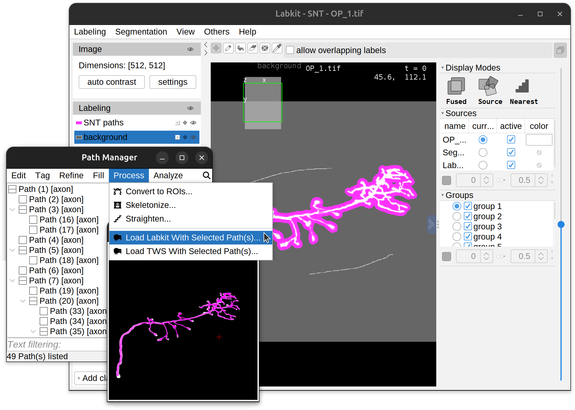 SNT Paths as classifier labels: Labkit. Drosophila OP neuron (3D grayscale image, demo dataset) being classified in Labkit.
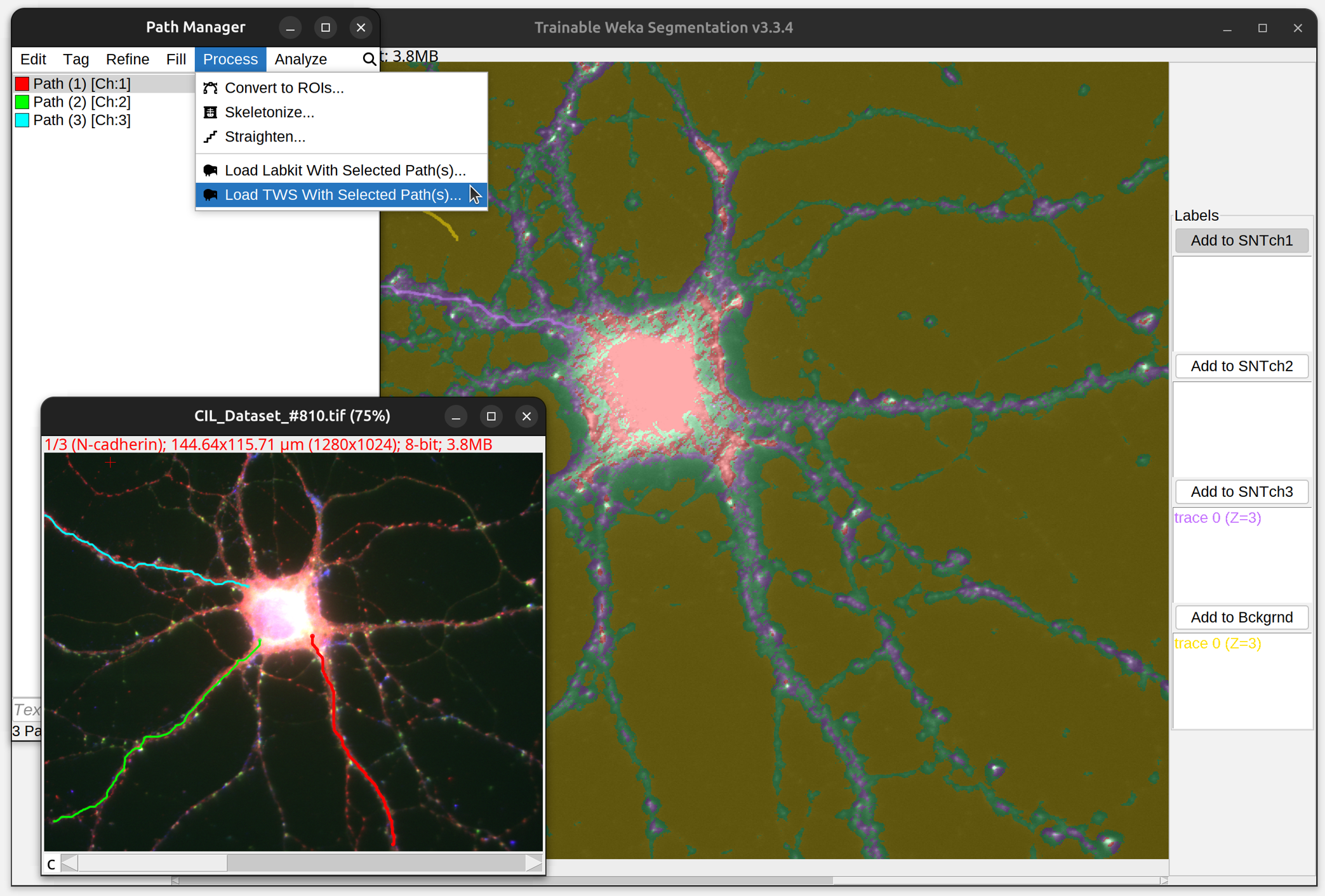 SNT Paths as classifier labels: TWS. A triple-stained neuron (2D multichannel image, demo dataset) being classified in TWS.
Scripts
There are a couple of examples in SNT’s neuroanatomy template collection handling image classification, namely:
- Apply Weka Model To Tracing Image: Demonstrates how to apply a pre-existing Weka model to the image being traced
- Train Weka Classifier: Exemplifies how to train a Weka model using traced paths and ROIs
Consuming DL Predictions
Probability Maps
A segmentation network’s per-voxel probability output can be loaded as a secondary tracing layer alongside the raw image. SNT’s autotracers can then use the probability map either as the primary signal (tracing directly on the network’s prediction) or as a score map that guides pruning and tip extension during autotracing (see Branch Filtering and Scoring). With semi-automated tracing, the secondary layer is opened using the Interactive Tracing widget in the Main tab. With auto-tracing, the score map is loaded/chosen as a parameter.
Note that any tool that can save a probability map (Labkit/TWS, custom PyTorch/TensorFlow scripts) is supported: SNT only sees the resulting image.
Seed Points
Many DL detectors output masks, or candidate locations: lists of soma centres, axon-terminal candidates, branch points, etc. SNT consumes these through the Seeded Tracing Assistant, where each candidate location/masked object lives as a 3D point with an associated confidence, optional radius, and free-form “type” and “source” fields. Once loaded, seeds can be:
- Filtered and curated interactively
- Used to root automated traces: E.g., cellpose masks can be used to specify the soma locations when autotracing multiple cells
- Used as endpoint targets for a single-cell trace
- Used as soft attractors that bias the routing of an automated trace through the predicted locations
See Seeded Tracing for full workflows. Note that the detector itself can be anything that produces a CSV list, or a labels image (from which centroids are extracted automatically).
Quality Control Locations
The Curation Assistant accepts DL-flagged “suspect” locations (e.g., from a model trained on previously-reviewed reconstructions) as warnings: each predicted location is shown in the Assistant’s warnings table for human review, mirroring how the Assistant’s own live monitors report issues from rule-based checks.
Programmatic entry is via CurationManager#addWarnings(List<Warning>). Each Warning is a record carrying a short check name, a severity (INFO, WARNING, ERROR), a human-readable message, an optional spatial location, the list of affected paths, and the measured value and threshold that triggered the entry. Once injected, predictions live alongside the Assistant’s own findings: they can be filtered by severity, navigated to on the canvas, tagged as accept / reject / unsure for downstream training, and visited in batch from the warnings table.
import sc.fiji.snt.analysis.curation.PlausibilityCheck.Warning
import sc.fiji.snt.analysis.curation.PlausibilityCheck.Severity
import sc.fiji.snt.util.PointInImage

// `predictions` is whatever a detector emits per suspect location
def warnings = predictions.collect { p ->
    new Warning("DL-QC", Severity.WARNING,
            "Predicted error (score=${p.score})",
            new PointInImage(p.x, p.y, p.z), // location
            p.nearbyPaths,         // List<Path> list of affected paths
            p.score, 0.5)          // measured value, threshold
}
ui.getCurationManager().addWarnings(warnings)
This turns the Curation Assistant into a generic target for any QC model that returns spatial predictions on a finished reconstruction, including models trained on the Seed Review export produced by an earlier curation pass, closing the feedback loop between review and retraining.
References
The Weka framework is described in:
- Eibe Frank, Mark A. Hall, and Ian H. Witten (2016). The WEKA Workbench. Online Appendix for “Data Mining: Practical Machine Learning Tools and Techniques”, Morgan Kaufmann, Fourth Edition, 2016. (PDF)