This page was last revised for version 5.0.0.
Measurements
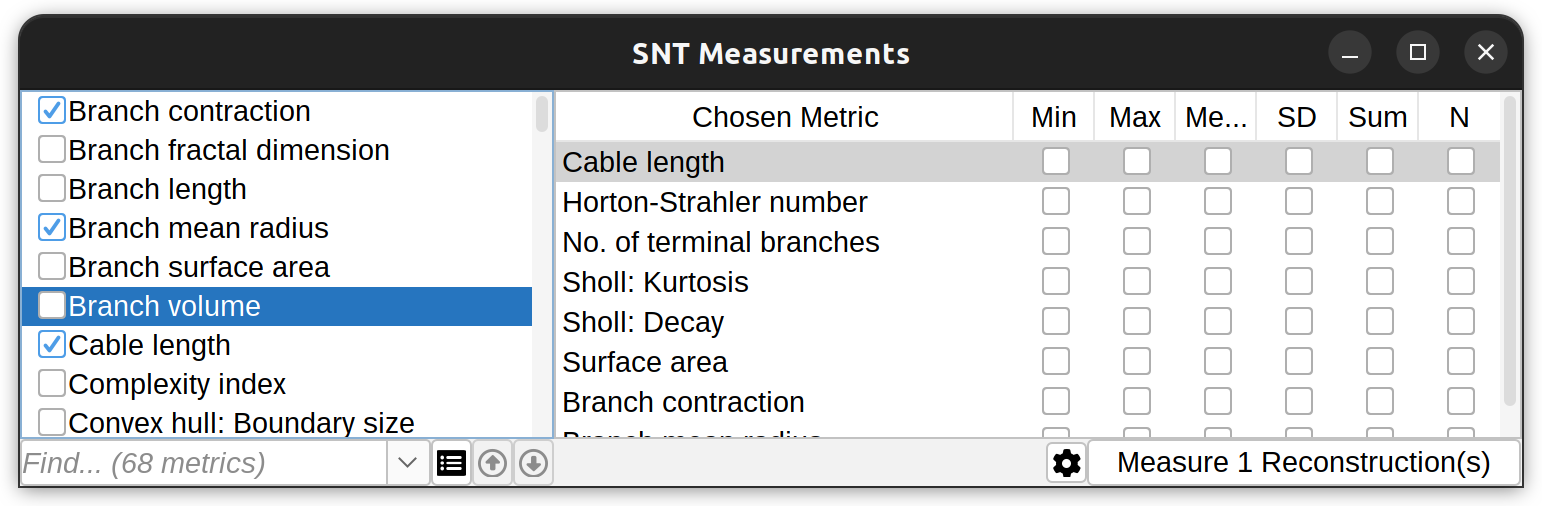
The measurements dialog features options for searching and selecting metrics, render measured cells, and summarize existing measurements. An offline guide is also accessible through the Gear menu.
SNT provides a couple ways to measure reconstructions. To measure complete cells use Analysis › Measure… in the main SNT dialog (or Analyze & Measure › in Reconstruction Viewer). To get measurements only on a select group of Paths, first select or filter for the Paths you want to measure in the Path Manager, then use the commands in Path Manager’s Analyze › Measurements menu.
The reason for distinguishing between cell-based (i.e., branch-based) and path-based measurements is flexibility: Path-based measurements can be performed on any structures, even those with loops, while cell-based measurements require the structure to be a graph-theoretic tree. The bulk of SNT measurements is described in Metrics. Measurements available in the GUI are typically single-value metrics. Many others measurements are available via scripting.
A convenience Quick Measurements command also exists ( Analysis › menu in the main SNT dialog or Analyze & Measure › in Reconstruction Viewer), in which common metrics are immediately retrieved using default settings without prompts.
Batch measurements of reconstructions can be accomplished via scripting. See, e.g., the bundled template script Measure_Multiple_Files.py, and related batch scripts for examples.
Note on Fitted Paths:
Some cell-based metrics may not be available when mixing fitted and un-fitted paths because paths are fitted independently of one another and may not be aware of the original connectivity. When this happens, metrics may be reported as NaN and related errors reported to the Console (when running in Debug mode).
If this becomes an issue, consider fitting paths in situ using the Replace existing nodes option instead. Also, remember that you can also use the Path Manager’s Edit>Rebuild… command to re-compute relationships between paths
Statistics
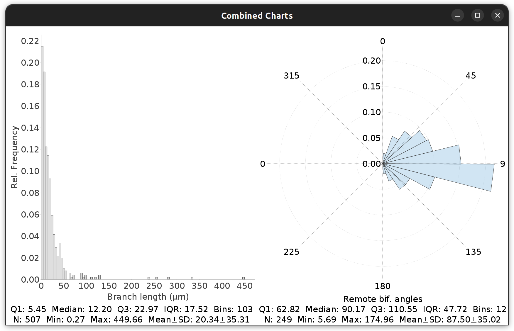
SNT assembles comparison reports and simple statistical reports (two-sample t-test/one-way ANOVA) for up to six groups of cells. This is described in Comparing Reconstructions. In addition, descriptive statistics are commonly reported in histograms from Frequency/Distribution Analysis commands.
Distributions or morphometric traits…
Notes on SNT charts and plots:
-
SNT charts are zoomable, scalable, and rendered using scientific plotting styles to be as publication-ready as possible. Right-click on a plot canvas to export it as vector graphics (PDF or SVG), access customization controls, a light/dark theme toggle, and options to aggregate charts in multi-panel figures
-
With simple charts, it is possible to double-click on plotted components to edit them and export data as CSV
-
Histogram distributions can be fitted to a normal distribution (Gaussian) or a Gaussian mixture model (see Components & Curve Fitting in the histogram right-click menu). In both cases, curves are scaled so that the area under the curve of the fitted curve matches that of the histogram. Quartile marks can also be overlaid. By default, the Freedman-Diaconis rule is used to compute the no. of histogram bins.
-
Unless specified, all radial plots display angles in [0°-360°[ degrees
-
While SNT is not a statistical analysis software, it does offer some basic convenience methods to parse third-party data. See e.g., this example for fitting a Gaussian mixture model to CSV data
Comparing Reconstructions
 SNT can compare up to six groups of cells. The entry point for this type of comparison is twofold:
- Utilities › Compare Reconstructions/Cell Groups… in the main SNT dialog. This includes a convenience option to compare single reconstruction files.
- Neuronal arbors › Load & Compare Groups… in Reconstruction Viewer, allowing groups to be tagged, and imported into a common scene while being compared.
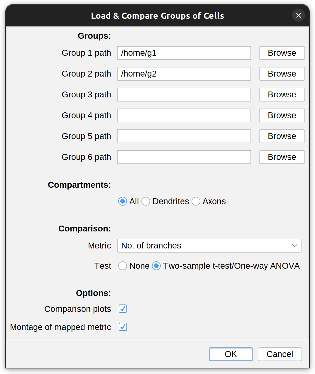
The dialog prompt for this feature allows selection of up to six directories containing reconstruction files (SWC, TRACES, JSON, NDF). The metric to compare against is chosen from the Metric drop-down menu. Optionally, it is possible to restrict the analysis to specific neurite compartments. After making your selections, press OK to run the analysis. The result typically includes:
- A simple statistical report, including descriptive statistics and a two-sample t-test (when comparing two groups) or one-way ANOVA (when comparing three or more groups)
- Comparison plots for the chosen metric: Grouped histogram and boxplot
- Montages of groups. These are multi-panel vignettes of up to 10 group exemplars. These can all be exported as PDF, PNG, or SVG
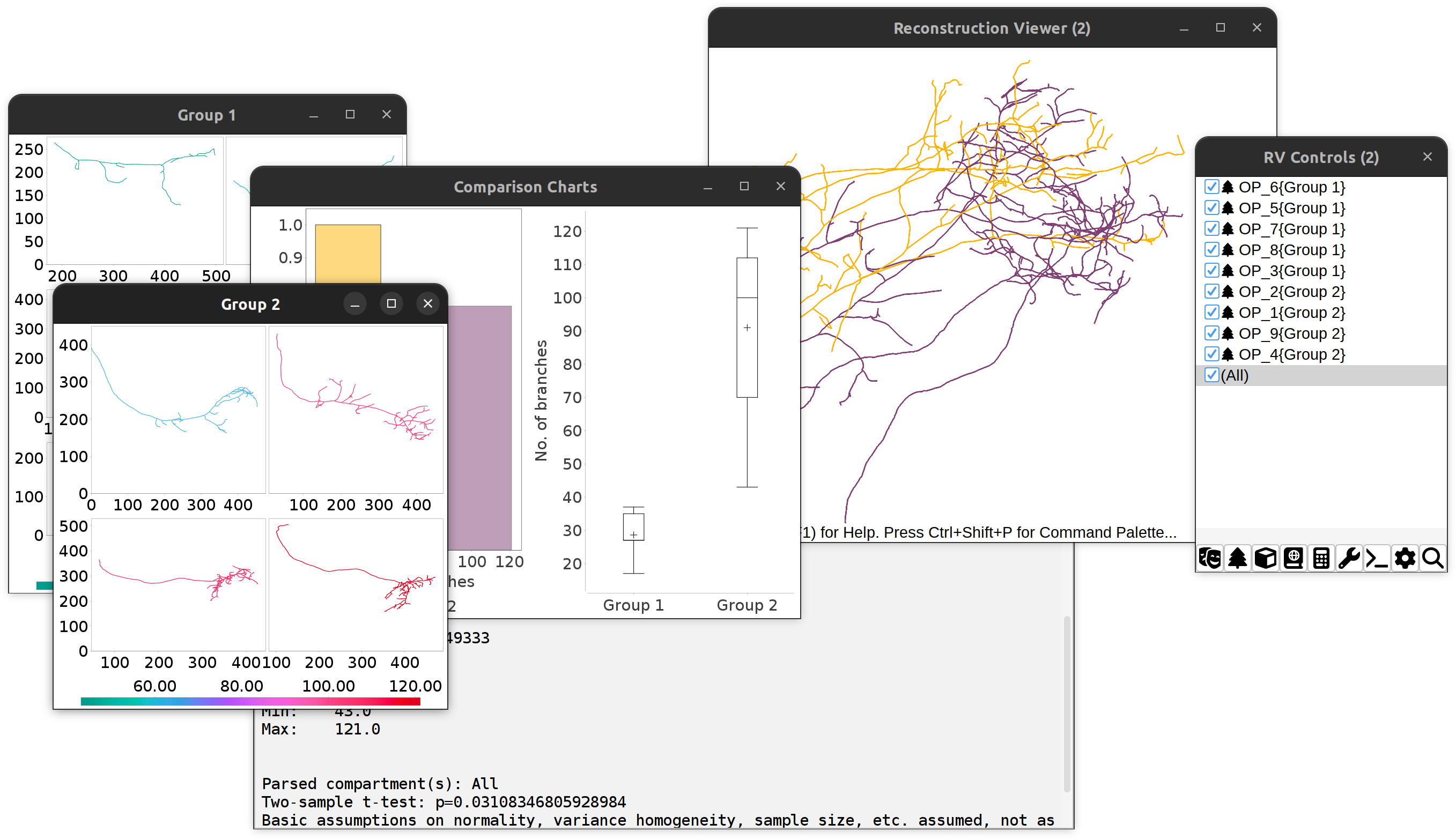
Comparing No. of branches between two cell groups: Overview of outputs.
SNT performs statistical tests without verifying if samples fulfill basic test-criteria (e.g., normality, variance homogeneity, sample size, etc.)
Convex Hull Analysis
Convex hull commands (in SNT main dialog, Rec. viewer and Rec. plotter) compute the 2D or 3D convex hull of a reconstruction (i.e., the smallest convex polygon/polyhedron that contains the nodes of its paths). Convex hull measurements are defined in Metrics.
Sholl Analysis
There are several entry points to Sholl Analysis in SNT. You can find those in the Neuroanatomy Shortcuts panel (Plugins › Neuroanatomy or “SNT” icon in Fiji’s toolbar):
- Sholl Analysis (Image): Direct parsing of images, bypassing tracing
- Sholl Analysis (Tracings): Parsing of reconstructions
- Sholl Analysis Scripts: These handle batch processing of files, specialized analysis, and misc. utilities
Sholl Analysis has a dedicated documentation page detailing parameters, plots, and metrics.
In the main SNT dialog, Sholl commands are available in the Analysis and image contextual menus and include:
-
Sholl Analysis… Analyzes cells based on a set of pre-defined, morphology-based focal points (e.g., Soma, Root node(s): Primary apical dendrite(s)). Note that this assumes the relevant morphology tag(s) have been assigned to the set of paths being analyzed. Since the center of analysis is only determined after the prompt has been dismissed, preview of sampling shells may not be available.
-
Sholl Analysis (by Focal Point)… Analyzes cells on an exact, user-defined focal point. It is described on the following section.
-
Sholl Analysis at Nearest Node Coarser alternative to Sholl Analysis (by Focal Point)…, run from the image contextual menu by right-clicking near a node (Shortcut: ⌥ Alt + ⇧ Shift + A.
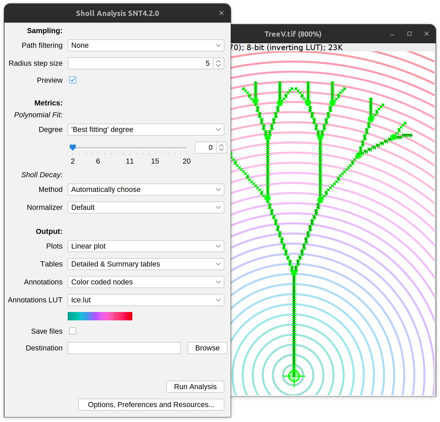
Sholl Analysis (by Focal Point)
For precise positioning of the center of analysis:
- Mouse over the path of interest. Press G to activate it
- Then, select the node to be used as focal point. This can be done in one of two ways:
- Select a node along the path as you would for forking operation: i.e., by pressing ⌥ Alt + ⇧ Shift while moving the cursor along the path (Note the “Fork Point” label appearing near the cursor on non-display canvases). With ⌥ Alt + ⇧ Shift still pressed, press A to start the analysis
- Make the path editable (right-click on the image and choose Edit Path from the contextual menu). Move the cursor along the path until the desired node is highlighted. Press ⌥ Alt + ⇧ Shift + A to start the analysis
NB: The default ⌥ Alt + ⇧ Shift modifier can be simplified in the Options tab of the main dialog.
The Sholl dialog created by this approach is a variant of the dialog created by running the Sholl › Sholl Analysis (From Tracings)… from the Neuroanatomy Shortcuts panel, with a couple of changes:
- Since the center of analysis is defined precisely on an image, radius step size can be previewed
- The Path filtering drop-down menu provides additional options to restrict the analysis to the subset of paths selected in the Path Manager
- The type of annotations is more specialized and includes:
- Color coded nodes Intersection counts will be color mapped into path nodes under the annotation LUT.
- 3D viewer labels image This generates a synthetic image holding the number of intersections at each distance from the center under annotation LUT. This image can then be fed to the “Apply Color Labels” action of the legacy 3D viewer, to “overlay” the mapping on the legacy 3D viewer scene.
Note that plots and tables can be directly saved to disk by selecting Save and specifying a valid directory in the dialog. The remaining options in the dialog are described in the Sholl documentation page.
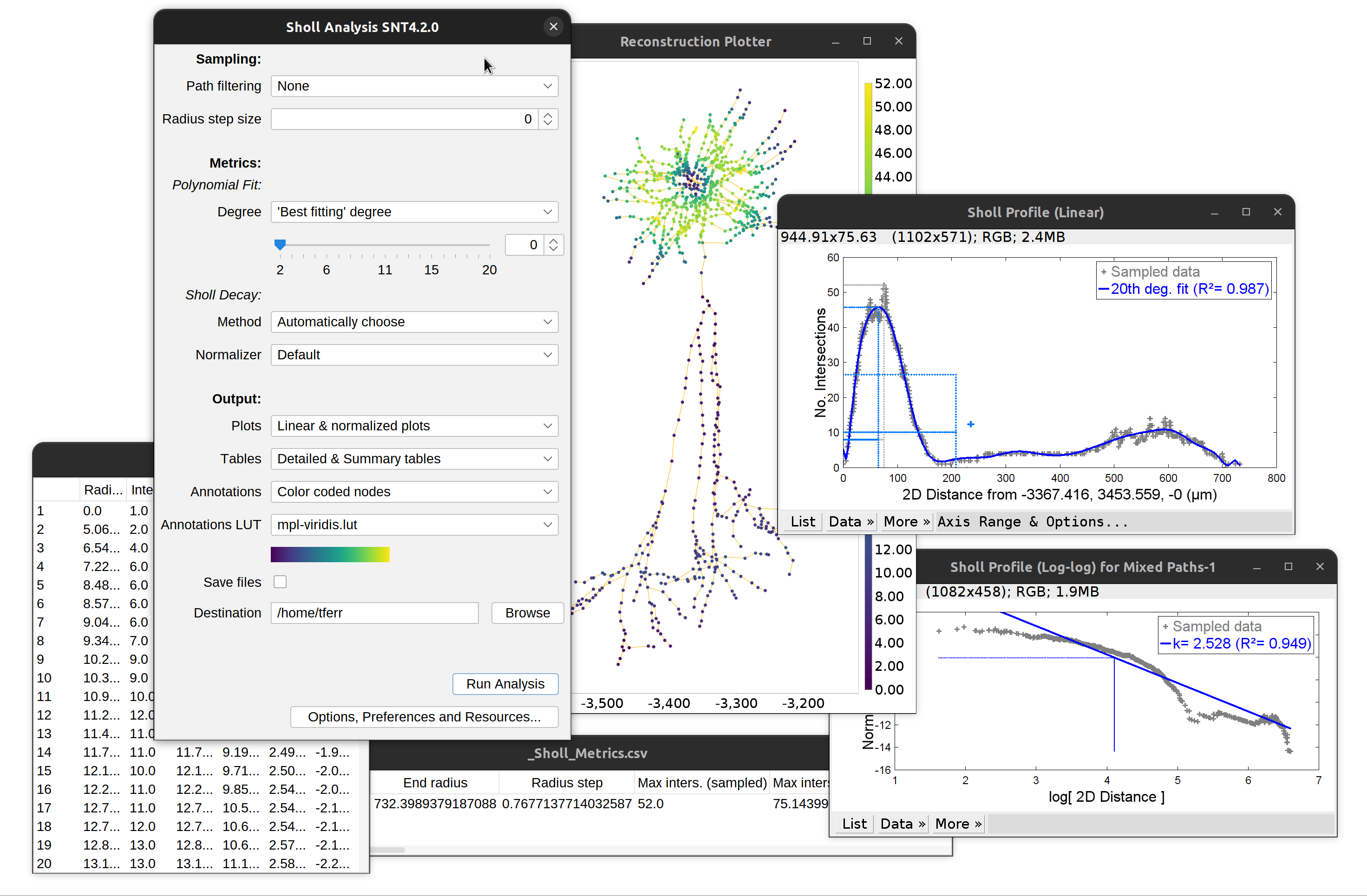
Overview of Sholl analysis outputs: Linear and log-log profile (Sholl decay calculation), detailed and summary tables. Note that ‘traditional’ plots are obtained by disabling curve-fitting altogether.
Strahler Analysis
Similarly to Sholl Analysis, there are several entry points to Strahler Analysis in SNT. You can find those in the Neuroanatomy Shortcuts panel (Plugins › Neuroanatomy or “SNT” icon in Fiji’s toolbar):
- Strahler Analysis (Image)… Direct parsing of images, bypassing tracing
- Strahler Analysis (Tracings)… Parsing of reconstructions (described in this section)
- Strahler Analysis Scripts: These handle batch processing of files
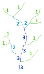
Strahler classification
Strahler numbering is a numerical procedure that summarizes the branching complexity of mathematical trees. The Strahler classification occurs as follows:
- If a branch is terminal (has no children), its Strahler number is one
- If a branch has one child-branch with Strahler number i, and all other children-branches have Strahler numbers less than i, then the Strahler number of the branch is i again
- If a branch has two or more children-branches with Strahler number i, and no children-branches with greater number, then the Strahler number of the branch is i+1
The Strahler number of a neuronal arbor reflects the highest number in the classification, i.e., the number of its root branch. Original publications by Robert E. Horton and Arthur N. Strahler include:
- Arthur N Strahler, Hypsometric (Area-Altitude) Analysis Of Erosional Topography (1952). GSA Bulletin; 63(11): 1117–42. doi: 10.1130/0016-7606(1952)63[1117:HAAOET]2.0.CO;2
- Arthur N Strahler, Quantitative analysis of watershed geomorphology (1957). Eos, Transactions American Geophysical Union, 38(6), 913–20. doi: 10.1029/TR038i006p00913 (PDF)
To conduct Strahler analysis on the current contents of the Path Manager, choose the Analysis › Strahler Analysis… in the main SNT dialog. This command will output the results of the analysis as a table and plot(s). These figures contain morphometric statistics (cf. Strahler metrics) of branches at each Horton-Strahler number.
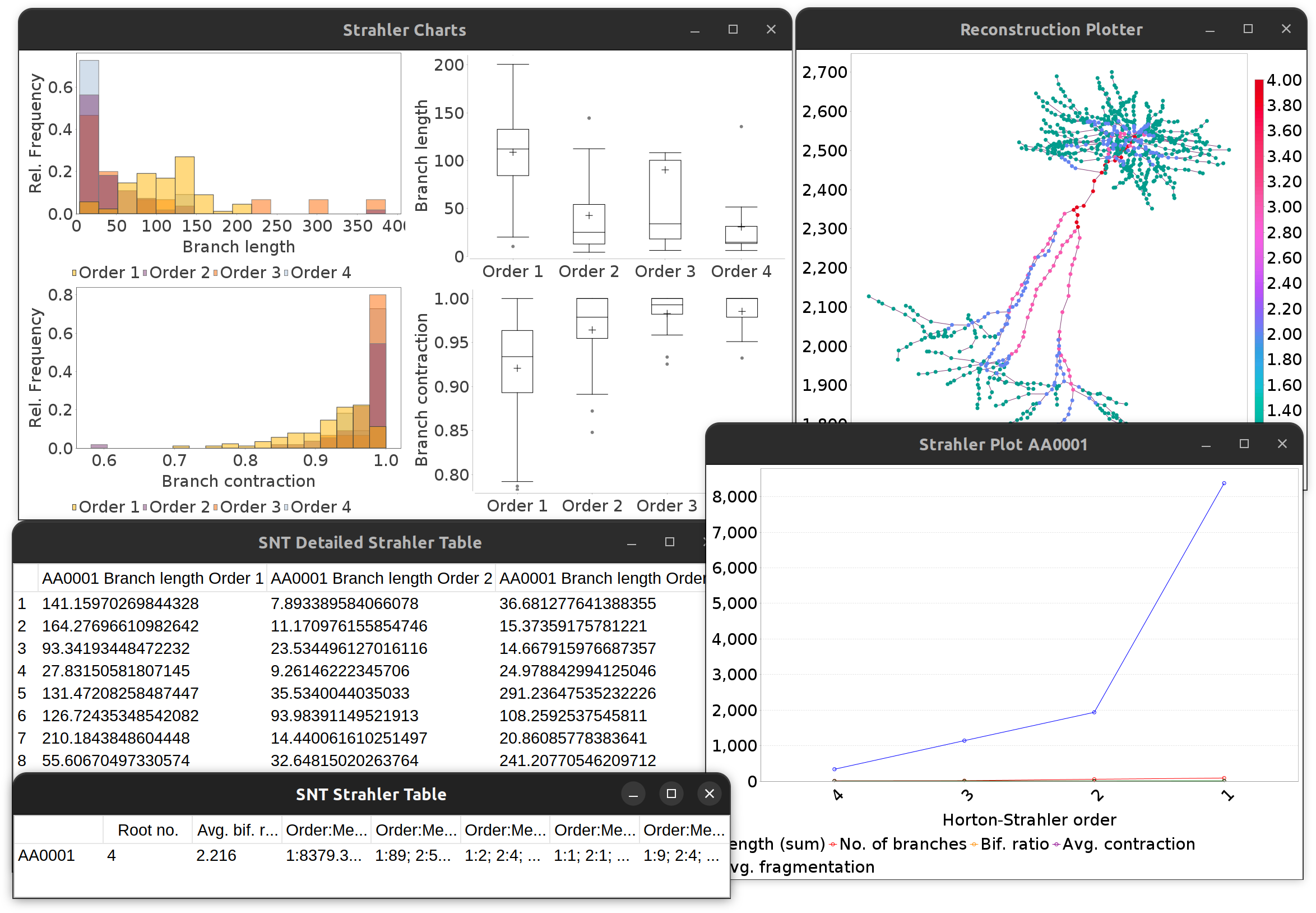
Strahler Analysis detailed output.
To conduct analyses directly from (thresholded) images, have a look at Strahler Analysis (From Images).
Path-based Analysis
Path-based analyses accept any traced structure (e.g., disconnected paths, paths associated with different cells, etc.), even those with loops. While most SNT measurements require traced structures to be valid mathematical trees, path-based measurements have no topological constraints. There are two commands in this category: Path Order Analysis, and Path Properties: Export CSV….
Path Order Analysis
This command (Analysis › Path-based › Path Order Analysis in the main SNT dialog) is a variant of Strahler with the following differences:
- Classification is based on Path Order: Paths are the scope of classification (not branches)
- Ranking of orders is reversed relatively to Strahler analysis (reversed Strahler orders), with primary paths having order 1 and terminal paths having the highest order
- Any collection of paths can be analyzed without validating into a formal tree
Path Properties: Export CSV…
This command (Analysis › Path-based › Path Properties: Export CSV…) exports path details (morphometrics, neurite compartments, linkage relationships to other Paths, start and end coordinates, etc.) to a spreadsheet file.
Atlas-based Analysis
Atlas-based analyses require reconstruction nodes to be tagged with neuropil IDs (atlas labels) (e.g., MouseLight data). Broadly, there are two types of analyses: Brain Area Frequencies and Annotations Graphs.
Brain Area Frequencies
This command (Analysis › Atlas-based › menu in main dialog, or Analyze & Measure › in Reconstruction Viewer) summarizes projection patterns across brain areas by computing frequency histograms of how often a morphometric trait (no. of tips, cable length, etc.) occurs across brain regions (neuropil labels). Such histograms can be obtained for groups of cells, isolated cells, or parts thereof.
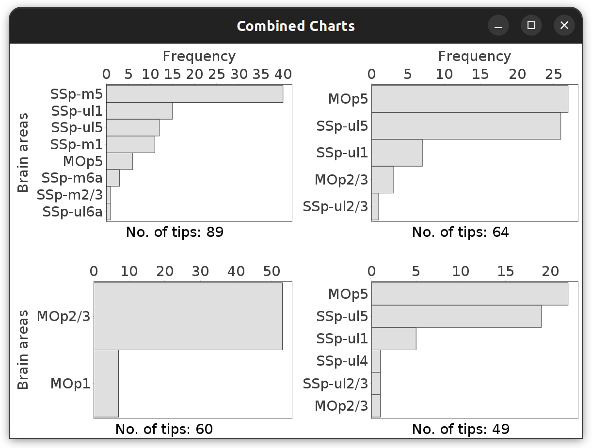 Brain Area Frequencies… in which No. of tips was tabulated across the motor cortex subregions associated with the four cells in the File › Load Demo Dataset… › MouseLight dendrites demo dataset
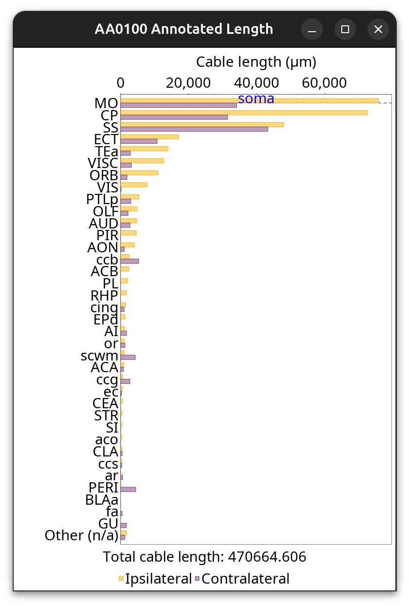 Brain Area Frequencies… of a single cell in which Cable length of axonal projections was tabulated across ipsilateral and contralateral hemisphere regions. See the Hemisphere Analysis notebook for details
Annotations Graphs
Annotations Graphs rely on brain annotations (i.e., neuropil labels) and are typically used to obtain unbiased, semi-quantitative summaries of projectomes or relationships between brain areas. Annotation graphs can be generated for a single cell or groups of cells. There are three major types of annotation graphs reporting neurite occupancy across brain areas/neuropil regions: 1) Sankey (flow) diagrams, 2) Ferris wheel diagrams, and 3) Boxplots:
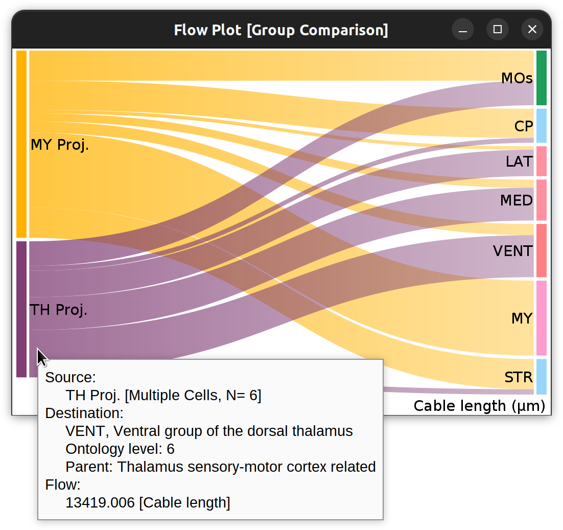 Flow-plot (Sankey diagram) for two groups of MouseLight PT-neurons: Medulla-projecting (MY Proj.) and Thalamus-projecting (TH Proj.) Flows depict axonal cable length (µm) at target areas (colored using the default ontology color-scheme adopted by the Allen Mouse Brain Common Coordinate Framework, CCFv3).
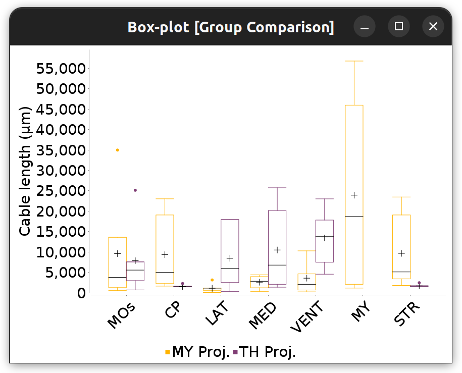 The same flow-plot data in boxplot format (see Flow and Ferris-Wheel Diagrams Demo script)
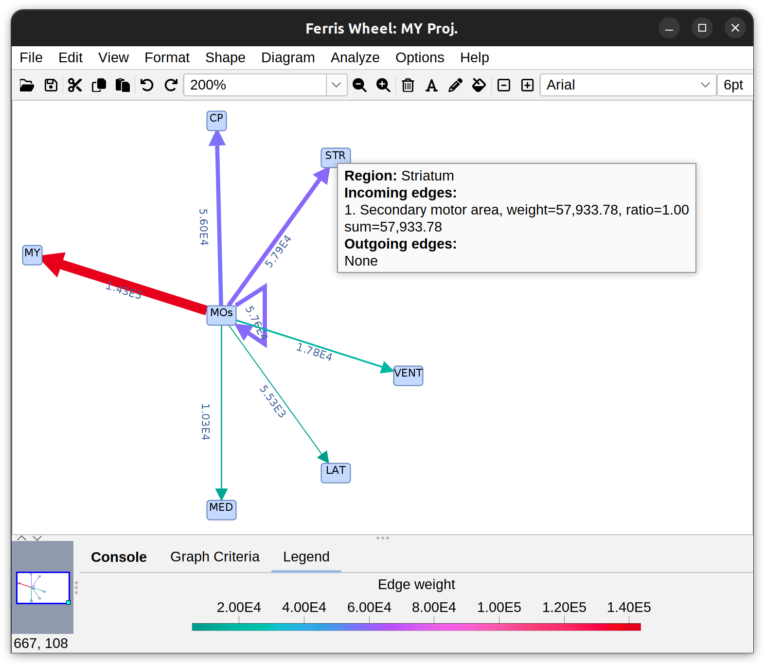 Ferris-wheel diagram for the group of MY-projecting neurons. These cells are located in the secondary motor cortex (MOs, center vertex). Outer vertices depict target areas innervated by the cells’ axons (automatically grouped by ontology). Edges encode axonal cable length (µm).
Prompts for generation of Annotation graphs, typically require a common set of inputs to be specified:
- Metric: The morphometric trait defining connectivity (cable length, no. of tips, etc.)
- Cutoff value: Brain areas associated with less than this quantity are excluded from the diagram. E.g., if metric is “No. of Tips” and this value is 10, only brain areas targeted by at least 11 tips are reported
- Deepest ontology The highest ontology level to be considered for neuropil labels. As a reference, the deepest level for mouse brain atlases is around 10. Setting this value to 0 forces SNT to consider all depths
Other types of specialized graphs are described in Graph-based Analysis.
Graph-based Analysis
Analyses based on graph-theory are better performed via the scripting. However, SNT features a quite-capable Graph Viewer that has many built-in options for handling graph objects.
The viewer provides controls for orientation, zoom level, panning, vertex editing and traversal as well as options to customize the display vertices (shape and labels) and edges (shape and weight labels). Basic support for themes (including dark, light and formal) are also supported. The Graph Viewer canvas may be exported in several file formats, including HTML, PNG, and SVG.
Typically, the most common types of graphs handled by Graph Viewer are:
-
Graphs based on morphology: Dendrograms can be obtained from single rooted tree structure, and provide a high-level overview of neurite branching topology. In the GUI, dendrograms can be created from Utilities › Create Dendrogram in the main SNT dialog or Analyze & Measure › Create Dendrogram in Reconstruction Viewer. Typically, dendrograms are generated for single cells
-
Graphs based on brain annotations As mentioned above, these rely on brain annotations (i.e., neuropil labels). Annotation graphs can be generated for a single cell or groups of cells
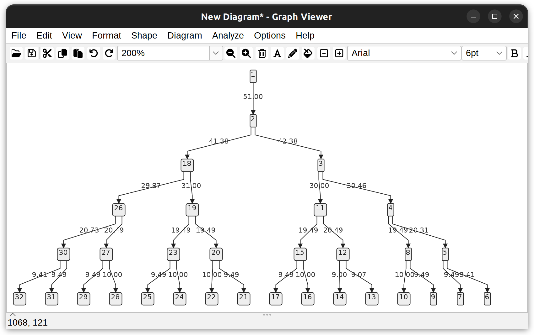 Dendrogram of a neuronal tree (Toy neuron demo dataset) under the vertical hierarchical layout. Edges depict branch length (µm). Vertices depict the root node (1), branch-, and end- points.
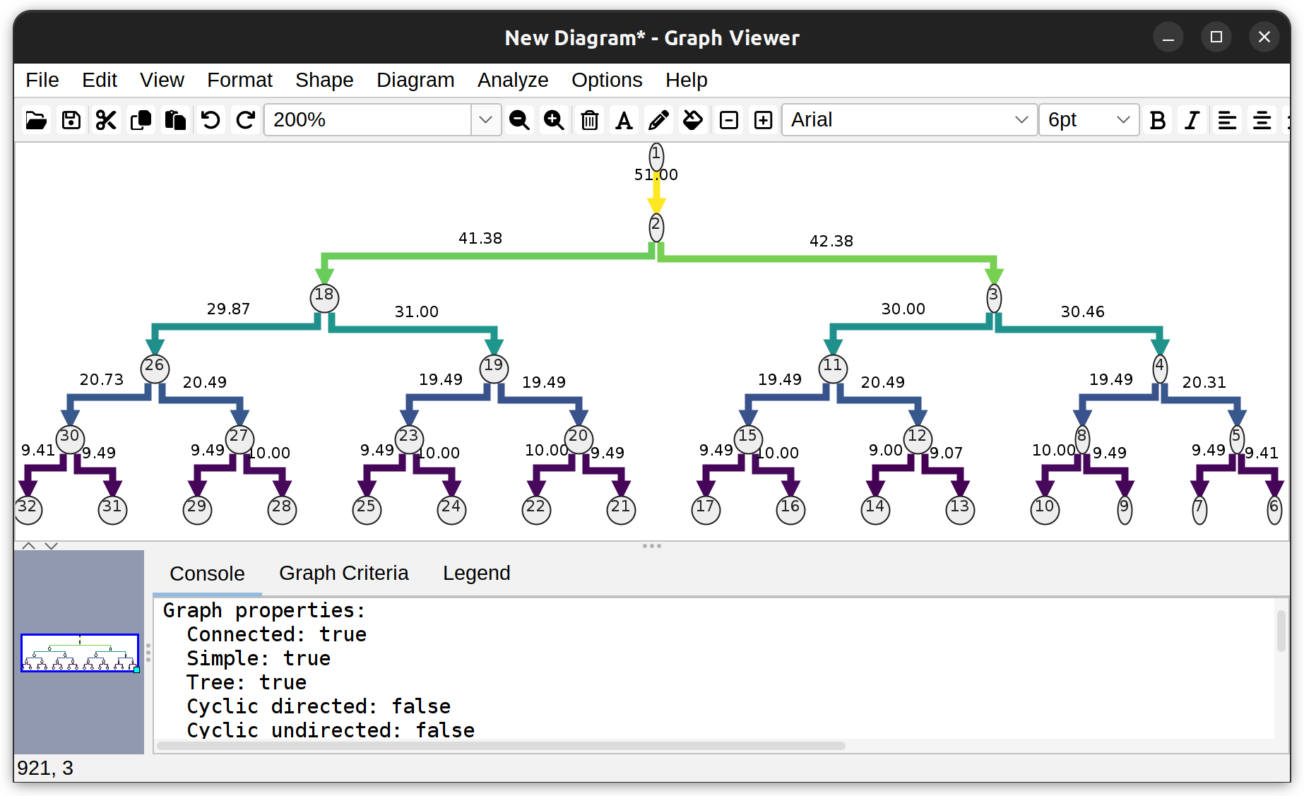 Dendrogram of a neuronal tree (Toy neuron demo dataset) color-coded by edge weight, i.e., branch length (µm), under the default layout (vertical tree).
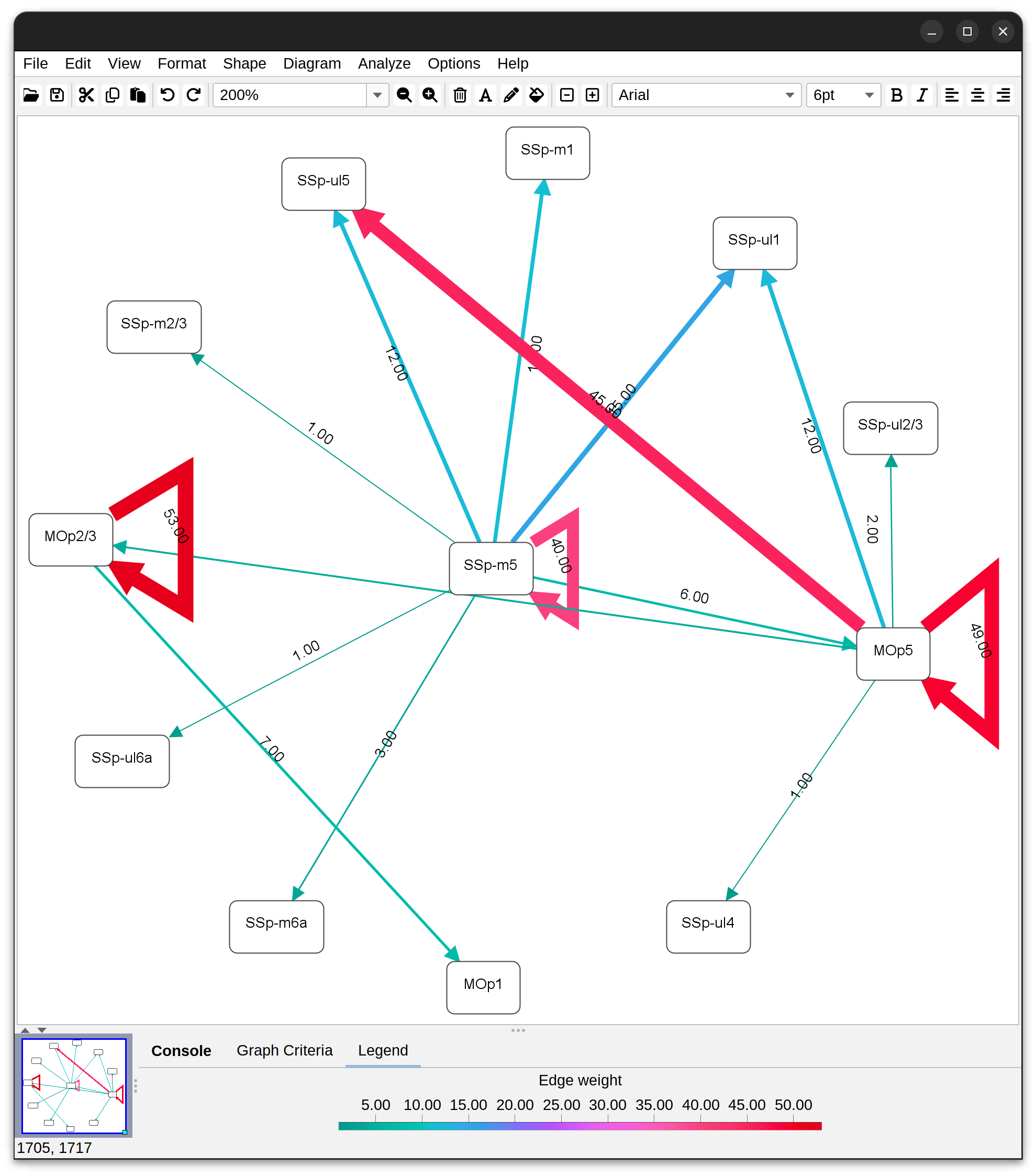 Relationships between brain areas associated with the MouseLight dendrites demo dataset
Ultimately, fine-grained programmatic control over SNT’s Graph objects is achieved via scripting. Relevant resources:
- JGraphT: The underlying library handling graph theory data structures and algorithms with JAVA and Python APIs
- SNT graph package: High-level tools for graph creation within SNT
- SNT Demo Scripts: See e.g., Graph_Analysis.py and Flow_and_Ferris-Wheel_Diagrams_Demo.groovy, two SNT demo scripts
- Python notebooks: For pyimagej examples, have a look at the Hemisphere Analysis notebook
Persistent Homology


Persistent homology computes topological features of neuronal reconstructions at different spatial resolutions, which in turn can be used to obtain topological signatures of their branching patterns. The Topological Morphology Descriptor (TMD) is the first published algorithm to use persistent Homology to describe neuronal arbors. It is described in:
Kanari, L., Dłotko, P., Scolamiero, M., Levi, R., Shillcock, J., Hess, K., & Markram, H. (2017). A Topological Representation of Branching Neuronal Morphologies. Neuroinformatics, 16(1), 3–13. doi:10.1007/s12021-017-9341-1.
SNT implements TMD and TMD variants by supporting several descriptor functions:
- Radial: The Euclidean (i.e., “straight line”) distance between a node and the tree’s root, as used in the original TMD description by Kanari et al.
- Centrifugal: The reversed Strahler classification of a node
- Geodesic: The “path distance” between a node and the tree’s root
- Path order: The path order of a node
- Coordinates: The X, Y, or Z coordinate of a node
In addition, SNT also implements descriptors based on persistence landscapes, as described in Bubenik, P. (2012). Statistical topological data analysis using persistence landscapes. ArXiv. doi:10.48550/ARXIV.1207.6437.
Currently, basic persistent homology descriptors can be computed using UI commands Analysis › Persistent Homology… (main interface), or Analyze & Measure › Persistent Homology… in Rec. viewer. Complete extraction of descriptors can be obtained with scripting. See e.g., the Persistence Landscape notebook tutorial.
Delineation Analysis
Delineations allow measuring proportions of reconstructions within other structures defined by ROIs or neuropil annotations (e.g., cortical layers, biomarkers, or counterstaining landmarks). Some of the questions that delineation analyses can answer include:
- Do branching patterns of neurons change along strata (cell layers)?
- Do branches near a lesion site differ from branches further away from it?
- Are there morphological differences across subregions of a neuron’s receptive field?
Delineations are described in Walkthroughs › Delineation Analysis.
Root Angle Analysis
Root angle analysis measures the angular distribution of how far neurites deviate from a direct path to the soma (or root of the neuronal arbor), a functional property that is captured by Sholl profiles (see also angular Sholl). It quantifies properties such as balancing factor, centripetal bias, and mean direction. It is described in:
doi:10.1016/j.celrep.2019.04.097
A root angle is defined as the angle between a neurite segment (defined centripetally from the termination point to the soma) and the direct path to the soma or root (see Bird and Cuntz 2019). The analysis proceeds as follows:
-
Root angles are computed centripetally for every node in the arbor in centripetal sequence (from tips to root)
-
The distribution of root angles is fitted to a von Mises distribution, a specialized probability distribution that models angles/directions. von Mises can be considered a ‘wrapped normal’, or a circular analogue of the normal distribution, as it addresses the issue of “wrapping” that occurs when dealing with angles revolving around a circle where 0° and 360° (2π) are the same.
-
Centripetal bias, Balancing factor, and Mean direction are then computed from the von Mises fit
The analysis can be performed from the Analysis menu in the main dialog, Reconstruction Viewer’s Analyze & Measure menu, or template scripts. The screenshot below depicts the output of the Analysis › Root Angle Analysis template script:
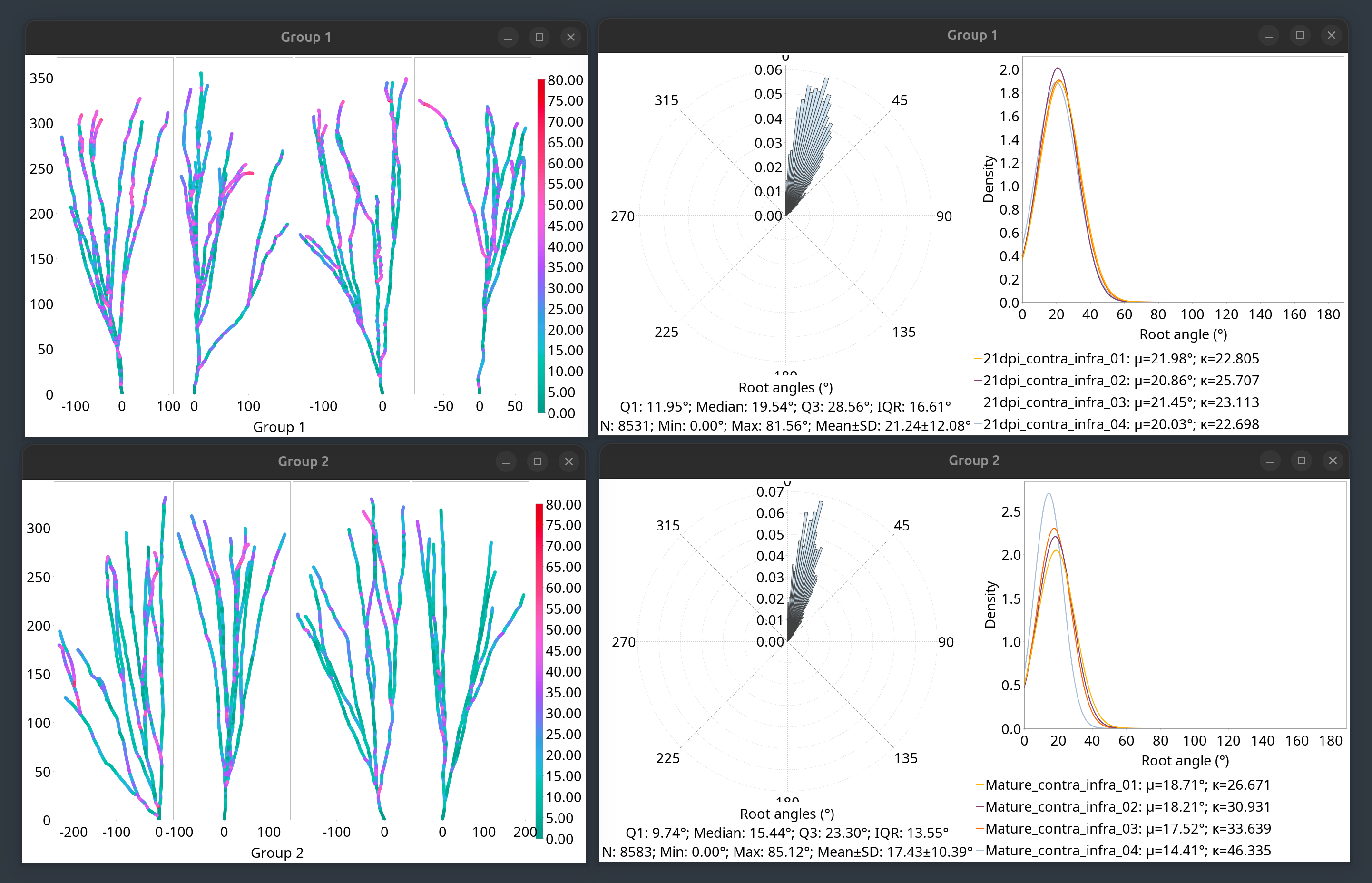
Root Angle Analysis outputs.
Growth Analysis
Growth Analysis provides detailed time-lapse analysis of neuronal patterns and requires traced paths to be matched across time frames, as detailed in the Time-lapse analysis walkthrough. The Analysis is accessed through the Path Manager’s Time-lapse Utilities menu.
For parameter validation and configuration comparisons, load the Hippocampal neuron (DIC timelapse) demo dataset (File › Load Demo Dataset…)
Prerequisites
- Time-matched paths: Paths must be tagged using the Match Paths Across Time… command first, so that all paths in the timelapse sequence associated with the same neurite are tagged with a common neurite label, e.g., “{neurite #1}”, “{neurite #2}”, etc, as described in the Time-lapse analysis walkthrough.
- Sufficient time points: At least 3 time points per neurite for meaningful analysis. Monitoring changes in extension angles typically requires at least 4 time points
Data generated outside SNT can also be analyzed:
- Import all the reconstruction files associated with the time series
- Apply “{neurite #}” tags using Match Paths Across Time…
- Run Growth Analysis…
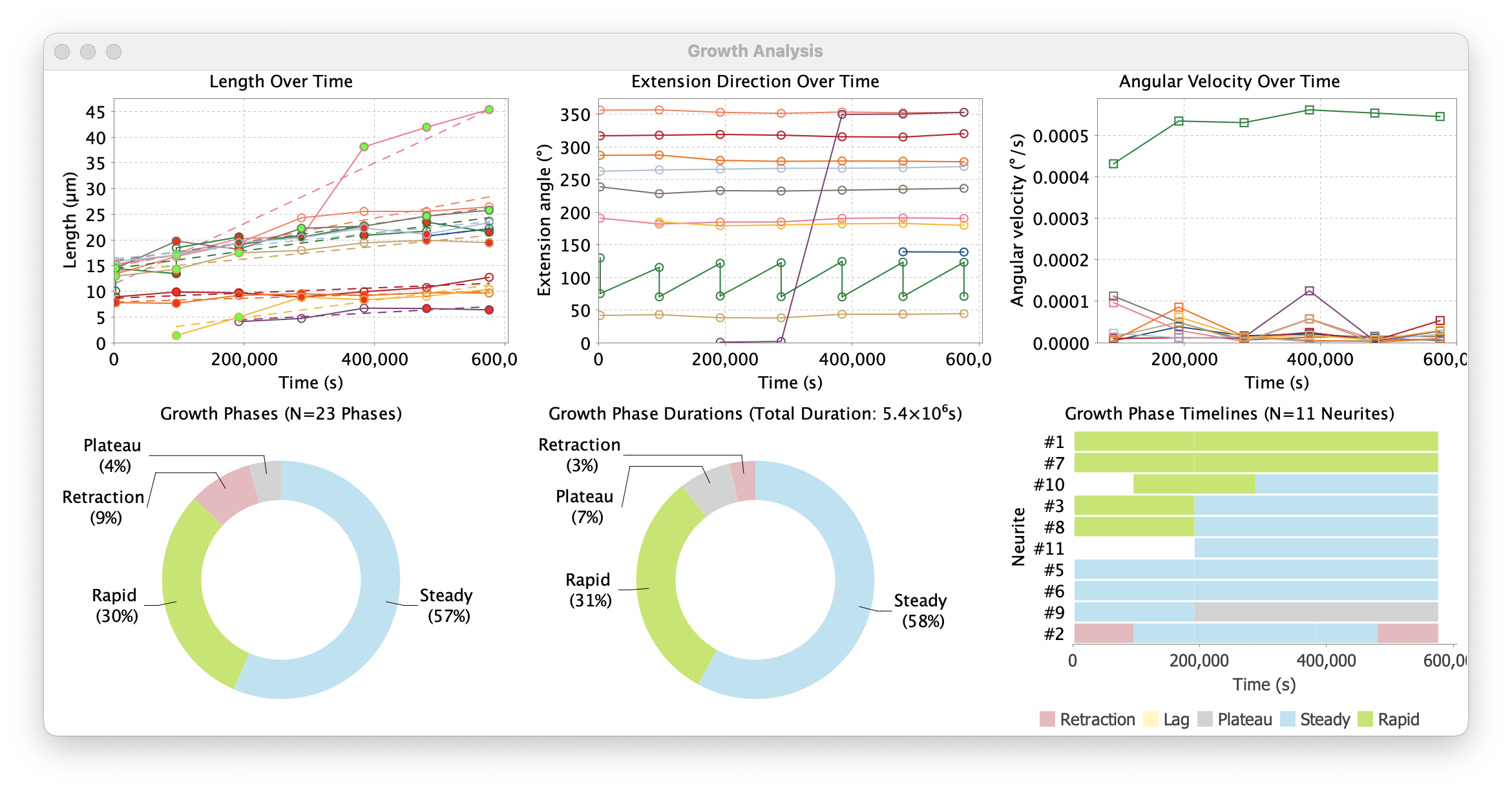
Growth Analysis outputs.
Classification Algorithm
The Growth Analysis… command classifies growth phases based on instantaneous growth rates relative to the overall average growth rate of each neurite. Algorithmically, the classification works as follows:
-
The overall growth rate of a neurite is calculated to establish a baseline
- A moving window “glides” along the time sequence to identify phase transitions in growth data. The detection combines three different detection methods to more robustly identify where changes in growth patterns occur. These include:
- Mean shift detection: Aimed at detecting sudden changes in average growth rate. This is usually effective at detecting Lag → Rapid; Rapid → Plateau; and Steady → Retraction transitions (see below)
- Variance change detection: Detects changes in growth rate variability, e.g., transitions from stable to variable growth
- Trend change detection: Detects changes in growth acceleration/deceleration patterns
- Growth rates are then split into five growth categories or phases:
| Phase | Definition | Interpretation |
|---|---|---|
| Retraction | Phase rate less than -min% of overall growth rate | Active shrinkage |
| Lag | Phase rate ≤ min% of overall growth rate | Slow growth |
| Plateau | Absolute value of phase rate < min% of overall growth rate | Minimal net growth |
| Steady | Phase rate within min% - max% of overall growth rate | Moderate growth |
| Rapid | Phase rate > max% of overall growth rate | Fast extension |
With overall growth rate, phase rate, and thresholds defined as:
| Term. | Definition |
|---|---|
| Overall growth rate | The slope of the linear regression fitted to the entire time series of length measurements. It represents the average rate of length increase over the complete observation period |
| Phase rate | Average of instantaneous rates within phase boundaries, with Instantaneous rate defined at each time point t as (length[t+1] - length[t]) / (time[t+1] - time[t]) |
| min% and max% thresholds | The cutoff thresholds ensure that e.g., fast-growing neurites aren’t misclassified as always “Rapid” or slow-growing neurites aren’t misclassified as always “Lag”. The min% cutoff represents the noise floor for growth measurements, while max% the cutoff threshold for significant acceleration. Cutoff thresholds can be calculated globally or relative to each neurite’s overall growth rate |
Outputs
-
Growth Phase Timeline: Temporal visualization of growth phases. This is a timeline chart showing the temporal progression of growth phases for each neurite. Each neurite is represented as a horizontal row with color-coded segments indicating different growth phases over time
-
Length Over Time: A scatter plot with trend lines showing the growth trajectories of individual neurites over time. Each neurite is represented by a colored line connecting measured length values at different time points
-
Phase Distributions: Statistical summary of phase types. These are two donut (ring) plots summarizing growth phases across all analyzed neurites. The “Growth Phases” plot summarizes the relative frequency of different phases, while the “Growth Phase Durations” plot summarizes cumulative durations
-
Angular Velocity Over Time: Angular velocity is the rate of change of angular position over time. It measures how quickly a neurite’s extension direction is changing over time. This type of data informs on how often a neurite changes direction, and how stable their directed growth is
-
Extension Direction Over Time: Absolute extension angles of neurites across time
-
Summarized Measurements: Tabular values of plotted data
Input Parameters
 The algorithm has several adjustable parameters that can be set in the “Growth Analysis…” prompt:
-
Threshold for ‘Lag/Plateau’ phase (%): Defines the minimum growth rate threshold for classifying growth phases. Growth rates below this threshold are classified as Lag or Plateau. Calculated as a percentage of each neurite’s overall linear growth rate. Lower values allow for detection of subtle growth variations, while high values detect only clearly distinct slow phases. Range: 10% - 50% (default is 30%)
E.g., For a neurite with an overall growth rate of 2.0 μm/m: With a 30% threshold, growth below 0.6 μm/m (2.0 x 30%) would be classified as Lag/Plateau.
-
Threshold for ‘Rapid’ phase (%): Defines the minimum growth rate multiple for classifying Rapid growth phases. Growth rates above this multiple of the overall rate are classified as rapid growth. Calculated as a percentage of each neurite’s overall linear growth rate. Lower values allow for detection of moderate growth accelerations, while high values detect only very fast accelerations. Range: 110% - 300% (default is 150%)
E.g., For a neurite with an overall growth rate of 2.0 μm/m: With a 150% threshold, growth above 3.0 μm/m (2.0 x 150%) would be classified as ‘Rapid’.
-
Threshold calculation: Either “Global” or “Per-neurite”. If global, thresholds are calculated relative to mean growth rate of all neurites. If “Per-neurite”: Thresholds are calculated relative to each neurite’s individual growth rate
-
Phase detection sensitivity: Sensitivity ranges from 0.05 to 1.0 (default value is 0.5). Lower values correspond to higher sensitivity, detecting more phase transitions (resulting in shorter, more numerous phases). Higher values correspond to lower sensitivity, detecting fewer transitions (resulting in longer, fewer phases). Increase this parameter if too many short phases are being detected. Decrease it if obvious phase transitions are being missed
-
Window size (no. of frames): Controls the size of the “moving window” of the phase detection algorithm. Higher values provide more stable detection with fewer phases, while lower values detect more detailed changes but may include spurious transitions. Range 2-40 frames (default is 3)
-
Threshold for retraction length (%): Defines the minimum percentage decrease in neurite length required to classify a phase as a retraction event. It is calculated at the start of the potential retraction. Increase this threshold if spurious “retraction” classifications occur. Range: 1% - 50% (default is 5%)
E.g., A neurite is 100 μm long at a given frame and decreases its length to 94μm in the subsequent frame. That’s a 6% reduction: With a 5% threshold, this change would be classified as “retraction”.
-
Filtering options: Filtering options are optional but may be useful for noisy datasets:
- Minimum length: Neurites that never reach this length throughout the timelapse are ignored. It allows very short paths to be excluded from analysis
- Minimum duration: Neurites extending for less than this duration are ignored. Allows short-lived neurites to be excluded from analysis
Other Specialized Analyses
See SNT Scripting, as well as script templates demonstrating a range of analysis possibilities.