This page describes a detector module for TrackMate that relies on cellpose to segment cells in 2D. It is not included in the core of TrackMate and must be installed via its own update site. It also requires cellpose to be installed on your system and working independently. This tutorial page gives installation details and advices at how to use the cellpose integration in TrackMate.
There are other TrackMate detectors shipped in the same update site, and documented separately:
- This page documents using cellpose 3.1.1 with TrackMate.
- There is also an advanced version of this detector, that let you configure additionnal parameters.
- The latest version of cellpose (as December 2025) is cellpose-SAM (cellpose 4), for which we made a specialized detector, documented here.
- Omnipose is another segmentation algorithm specialized for rod-shape bacteria. Because it is a based on Cellpose, its TrackMate integration is shipped in the same upate site and documented here, and here for its advanced version.
Cellpose is a segmentation algorithm based on Deep Learning techniques, written in Python 3 by Carsen Stringer and Marius Pachitariu. If you use the cellpose TrackMate module for your research, please also cite the Cellpose 3 paper:
doi:10.1038/s41592-025-02595-5
Installation
We need to subscribe to an extra update site in Fiji, and have a working installation of cellpose on your system.
TrackMate-Cellpose update site
In Fiji, go to Help › Update…. Update and restart Fiji until it is up-to-date. Then go to the update menu once more, and click on the Manage update sites button, at the bottom-left of the updater window. A new window containing all the known update sites will appear. Click on the TrackMate-Cellpose check box and restart Fiji one more time.
Conda & Cellpose
This step is completely independent of Fiji. If you have already a working cellpose installation, you can skip this section entirely. But we absolutely need a working cellpose.
There are many ways to get cellpose installed. We give a subset of them in the last section of this document.
Once this is done, TrackMate needs to know where you installed conda. You need to do this only once. This is documented on this page.
Usage
Cellpose parameters in the TrackMate UI
 We document these parameters from top to bottom in the GUI.
Conda environment
Specify in what conda environment you installed Cellpose (the v3.1.1 in the case of this detector). If you get an error at this stage, it is likely because the conda path for TrackMate was not configured properly. Again, check [this page]((/plugins/trackmate/trackmate-conda-path) if this happens.
Pretrained model
This list lets you select the pretrained models that were shipped with Cellpose 3. They are dully documented in details on the Cellpose doc website. The ‘main’ ones are:
- the
cyto3model, that excels at segmenting cells stained for their cytoplasm. This model supports the specification of a second channel (see below) where nuclei are stained, to guide cell sgmentation. - the
nucleimodel, trained to segment cell nuclei.
Path to custom model
There are radio buttons before the Pretrained model and Path to custom model that lets you select whether you want to use a pretrained model, or a custom one.
When Path to custom model is selected, you need to browse to the actual model file.
Note that it must be the an absolute path to the file.
Target channel
If your image has several color channels, choose here the channel to segment. The number of the channel corresponds to the imagej channel in your image.
It should be the channel where the cytoplam staining is for cell segmentation, or the nuclei staining for nuclei segmentation, e.g. with the nuclei model.
Note that TrackMate doesn’t handle RGB stacks so you might need to convert your image if it is not already a composite image (see below for tip on how to pass RGB images to TrackMate-Cellpose)
Second optional channel
The cyto3 (and cyto2 and cyto) pretrained models have been trained on images with a second channels in which the cell nuclei were labeled. It is used as a seed to make the detection of single cells more robust.
It is optional and this parameter specifies in which channel are the nuclei (the number of the imagej channel of the nuclei). Use ‘0’ to skip using the second optional channel.
For the nuclei model, this parameter is ignored.
Cell diameter
cellpose can exploit an a priori knowledge on the size of cells. If you have a rough estimate of the size of the cell, enter it here. In TrackMate this parameter must be specified in physical units (for instance µm if the source image has a pixel size expressed in µm). Enter the value ‘0’ to have cellpose automatically determine the cell size estimate.
Careful! I insist a bit on this point. If you are used to running Cellpose from the Cellpose UI or a Python script, it expects the diameter to be in pixels. But here in TrackMate, the diameter is in the spatial units of your image.
Use GPU
If this box is checked, the GPU will be used if cellpose was installed with required librairies and hardware to use the GPU. If the GPU support is absent or incorrect, this setting will be safely ignored and the computation will rely on CPU only. Unchecking the box will force cellpose to use the CPU even if GPU support is available.
We took special care to implement multi-threaded processing if you use CPU. With this setting, there will be one Cellpose process running per thread you set in the Edit > Options > Memory and Threads… configuration (“Parallel Threads for stacks”). And then each image corresponding to the time-points will be dispatched automatically to these multiple processes, running concurrently.
Simplify contours
If this box is checked, the contour outlines generated by the masks returned by cellpose will be smoothed and simplified. This is the same treatment that is used by other TrackMate detectors and documented here.
(Re)Training of a cellpose model
To optimize CellPose on your data, you can retrain one its model and use it in TrackMate-CellPose. You can do the retraining easily through CellPose 2.0 GUI. When the model gives acceptable results, select it in TrackMate interface with the Path to custom model parameter.
Tutorials
Tracking cells stained for cytoplam with cellpose
One of the central advantage of cellpose is its ability to give robuset segmentation results for cells stained for cytoplasm. We will use such a movie in this tutorial. You can download the movie from Zenodo:
![]()
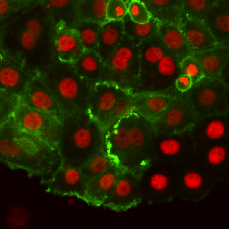
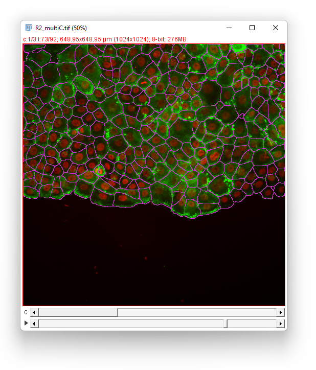
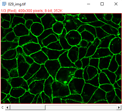
These are breast cancer cells moving collectively. We are tracking them to analyze how their migration parameters change in various conditions.
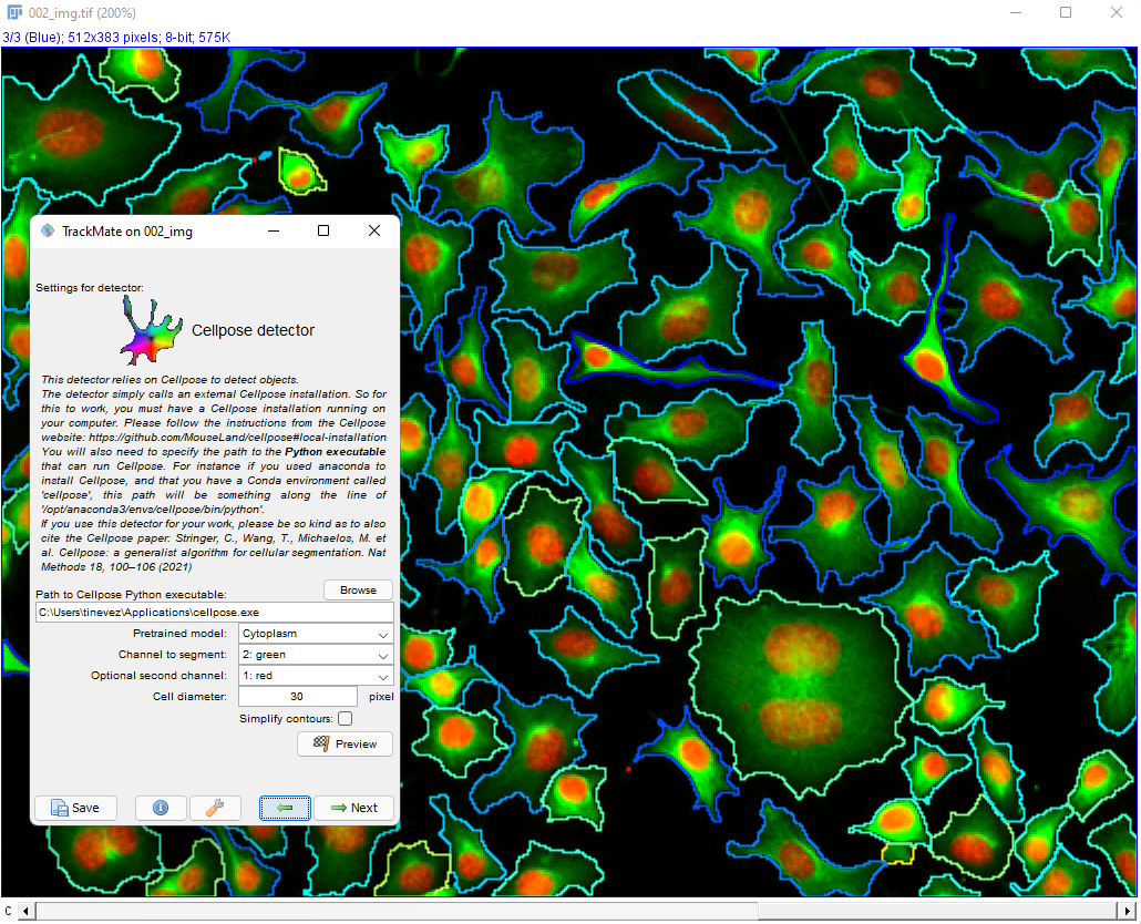
The movie comes from RGB images that have already been split in 3 separated components. The blue channel is empty. The red channel display the cell nuclei. The cells are stained for cytoplasms in the green channel, with a lot of variability from one cell to another. The texture and sometimes the intensity hints the cell border. This is an image that would be considered very hard to segment with classical techniques.
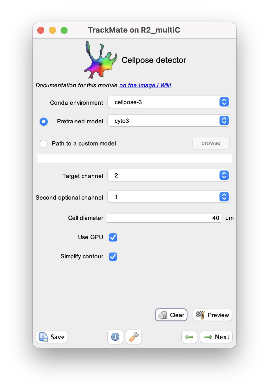
Open Fiji and load the image. Then launch TrackMate in Plugins › Tracking › TrackMate. In the second panel, select the cellpose detector:
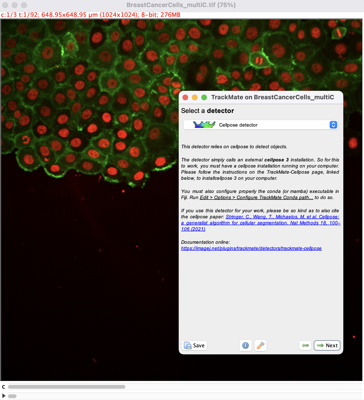
then click the Next button. You should see the configuration panel for cellpose.
On the Conda environment select the name of the environment Cellpose 3 is installed (cellpose-3 in the example above).
We want to segment the touching cells and obtain their contour. So we will use the cyto3 model, to be selected in the Pretrained model list.
The cytoplasm is imaged in the second channel (it happens to use the green LUT, but it would not matter) so we enter 2 for the Target channel parameter.
The channel 1 contains the nuclei so we can specify it in the Second optional channel parameter.
Finally, we can measure a rough estimate of the cell size using ImageJ ROI tools, which is about 40 µm, and enter this value in the Cell diameter field.
The movie is quite big, and will take several minutes to process using only the CPU (on my Mac it takes about 20 minutes without multithreading). Having a cellpose installation with GPU support really accelerate segmentation.
Finally, for this movie we want the cell contour to follow the pixels of the masks generated by cellpose, so we unchecked the Simplify contour box.
Then we are ready to launch segmentation. Click the Next button. The log window will echo the messages from cellpose. On a windows machine with GPU support, the detection step takes about 2 minutes.
On a 2022 MacBook Pro using GPU, it takes about 4 minutes.
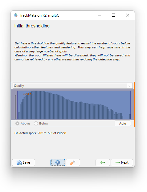
The Initial thresholding reports the quality histogram for all detections. Here, the quality is just the area of detections in pixel units. We see that there are some detections with very little size, probably for spurious objects. We can filter them out by setting a threshold value around 220.
Click the Next button. In the Spot filter panel TrackMate first computes all the spot features. Then the results are shown. Given the difficulty of the segmentation task, the results are surprisingly good, and we should thank cellpose for it. They are not perfect though. For some big and faint cells, we can see a few events of oversegmentation, probably caused by red granules drifting in some cells. Still, we can follow cell division by eye and see that the vast majority of them is detected properly.
We don’t need to filter the detections so click the Next button. Our aim is to detect cell divisions as they migrate, so we have to pick either the LAP tracker of the Overlap tracker. Given the cell density we would normally use the LAP tracker. However it would introduce too many false positive in the cell division detection. Indeed, the cells migrate “downwards” in the image, and new cells appear in the field-of-view from the top of the image. These new cells would be elected as candidates to be the daughter emerging from a non-existent division of the cell just below it. The overlap tracker will be more robust against this artifact so we elect to chose it.
We use the following parameter:
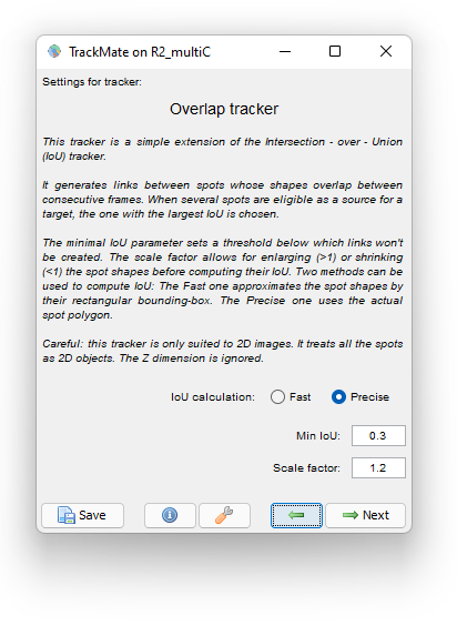
We dilate the cells with a Scale factor of 1.2 so that if the daughter cells moved away from the mother cell they are still linked to the mother. A Minimal IoU value of 0.3 mitigate false cell division detections. Choosing the Precise method for IoU calculation has some cost on tracking time (5 s. versus 1 s. for the Fast method) but it is so short in our case that we still use it.
Here is what the tracking results look like:
In the movie above the cells are colored by their track ID, which tends to highlight tracking mistakes and missed detections. Indeed, some cell divisions are missed. Still the results are better than what they would be with the LAP tracker, due to the bias for low Y value discussed above.
Using a custom cellpose model to track cells imaged in bright-field
Another key advantage of cellpose is that it is relatively easy and fast to train or augment a model to harness difficult use cases that are not handled well by the pretrained model.
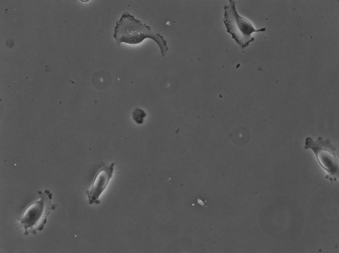
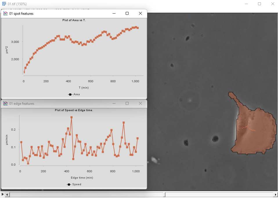
For instance the cells above were imaged in bright-field at high resolution. They are Glioblastoma-astrocytoma U373 cells migrating on a polyacrylamide gel. They have a rather complex shape and a low contrast. The segmentation of cells in such images is normally difficult with classical image processing techniques. In the following we will use the TrackMate-Cellpose intragration to segment and track them. Our goal is to see if we discriminate between two types of cell locomotion based on dynamics and morphological features of single cells. We will see how to give more robustness to the analysis by filtering out some detections close to image border.
The data can be obtained from Zenodo:
![]()
The dataset contains a custom cellpose model. We have trained a it using the ZeroCostDL4Mic platform. This cellpose model was trained for 500 epochs on 214 paired image patches (image dimensions: 520x 696), with a batch size of 8, using the Cellpose ZeroCostDL4Mic notebook (v 1.13). The cellpose cyto2 model was used as a training starting point. The training was accelerated using a Tesla K80 GPU.
To use the model you need to unzip the Cellpose model 171121-20211118T111402Z-001.zip file. The cellpose model file itself is the cellpose_residual_on_style_on_concatenation_off_train_folder_2021_11_17_19_45_23.398850 file in the 171121 folder.
We can use it in TrackMate by checking the radio button in front of the Path to a custom model parameter:
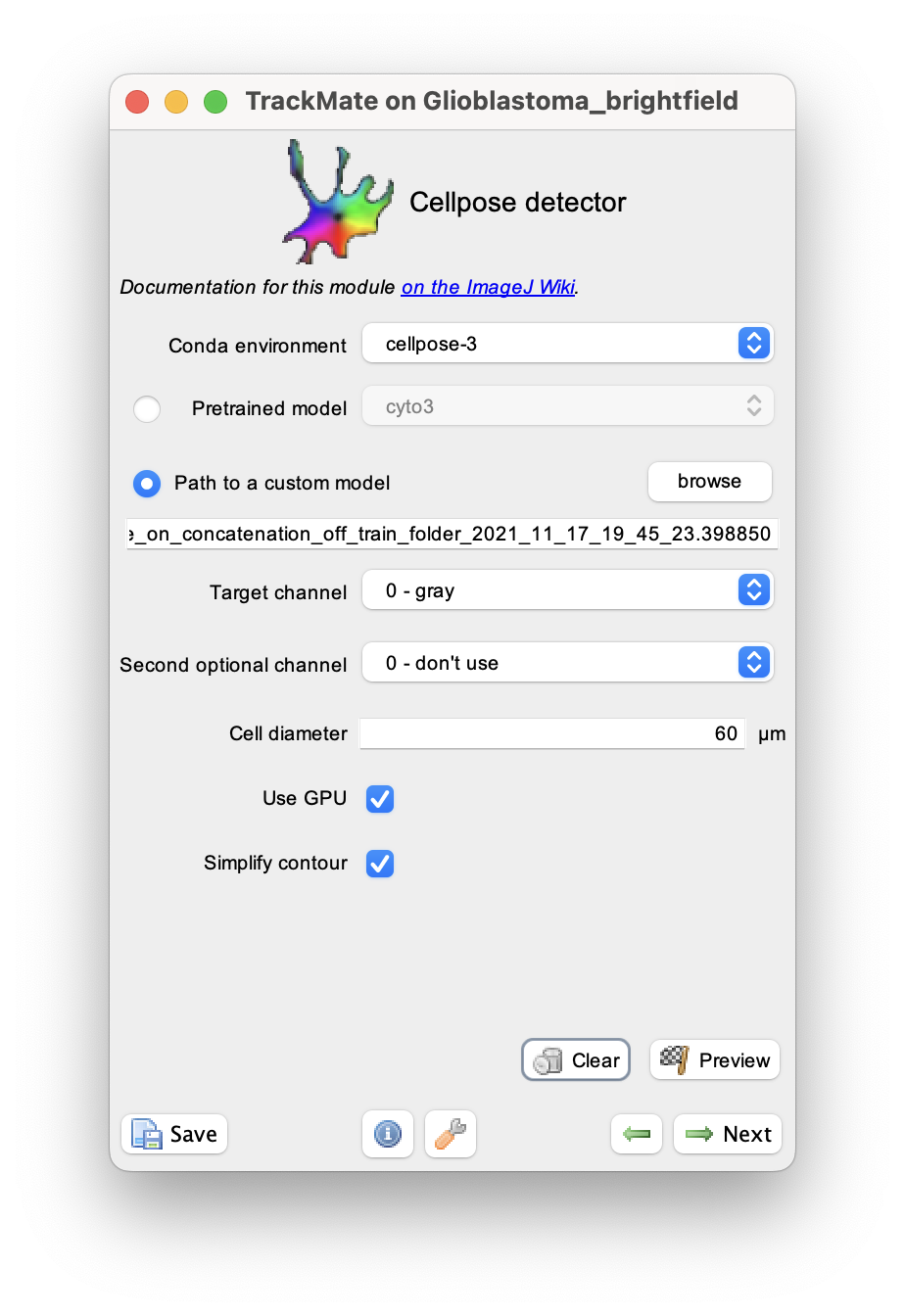
For the Path to a custom model parameter, I browsed to the model file (in this case, ending in .398850).
There is only one channel, so I used 0 for both the target and optional channels. The cell size measured with ImageJ is about 60 µm.
On a 2022 MacBook Pro used in this demo, the Cellpose installation have GPU support, so I left the corresponding box checked. Later we will measure shape descriptors for the cell, so it is important to simplify their contours, and the corresponding box is also checked.
Clicking Next starts the segmentation. In my case it completes in about 30 seconds. In the Initial thresholding panel, choose a threshold of 0 to include all detections in the next step. We get the following results displayed in the Spot filter panel:
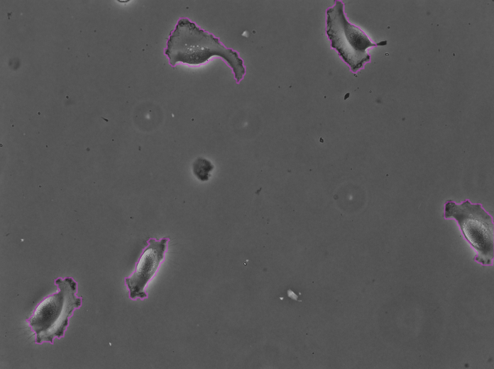
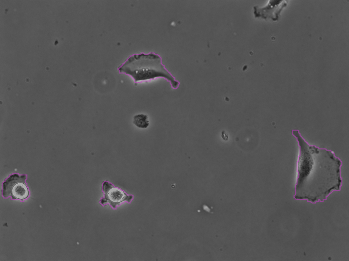
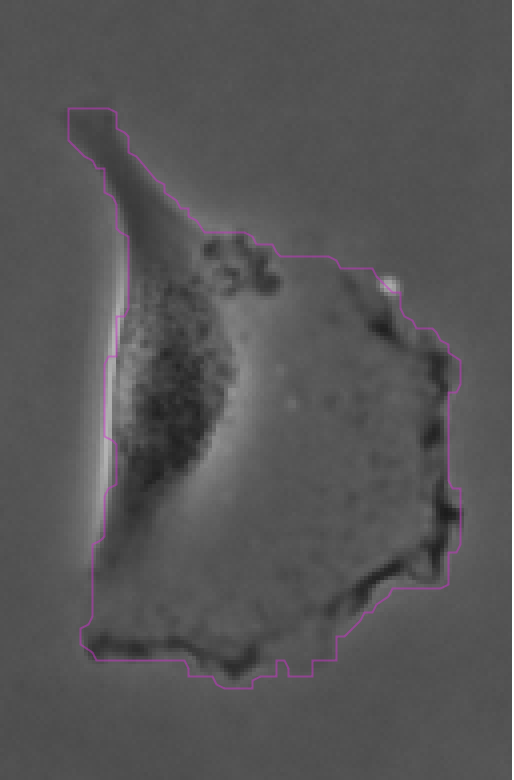
The contours are not absolutely perfect. In a few cases they miss a cell extrusion or include a debris that touches the cell. Some cells that touch the border of the image are not detected. But overall the results are very good and there is no spurious detection. We don’t need to add spot filters at tis step.
For this movie, the tracking part should be simple as the cells are well separated and move by a distance smaller than their size from one frame to the next. Yet, we have to bridge over the missed detections when cells were close to the border. The Simple LAP tracker is suitable for this case:
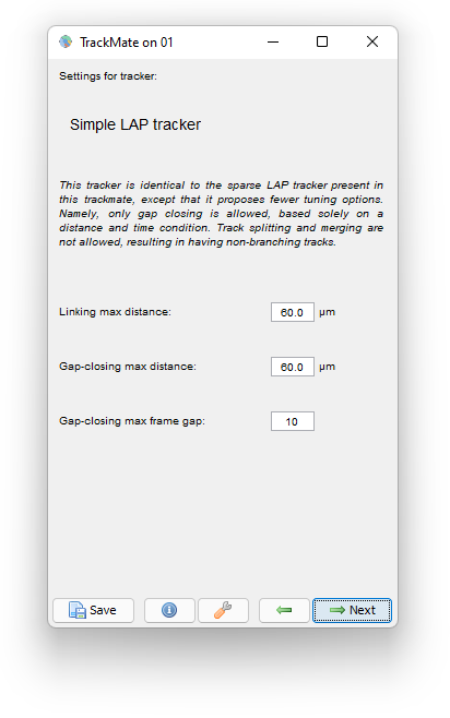
The max distance are taken from the cell size. Note the large max frame gap, chosen to accommodate several missed detections near the image borders. As final results we get:
We can distinguish roughly two modes of motion for the cells in this movie. The two cells in the bottom-left part of the image display saltatory movements with extrusion forming on changing sides of the cell, followed by a retraction and a large but brisk movement of the nucleus. The other cells display a large lamellipodium and exhibit a smooth motion in the direction of the protrusion.
We can use the Plot features panel to investigate these behaviors quantitatively. For instance, one of the two cells in the bottom-left (in blue in the movie above and in the figure below) display this dynamics for the cell area and speed:
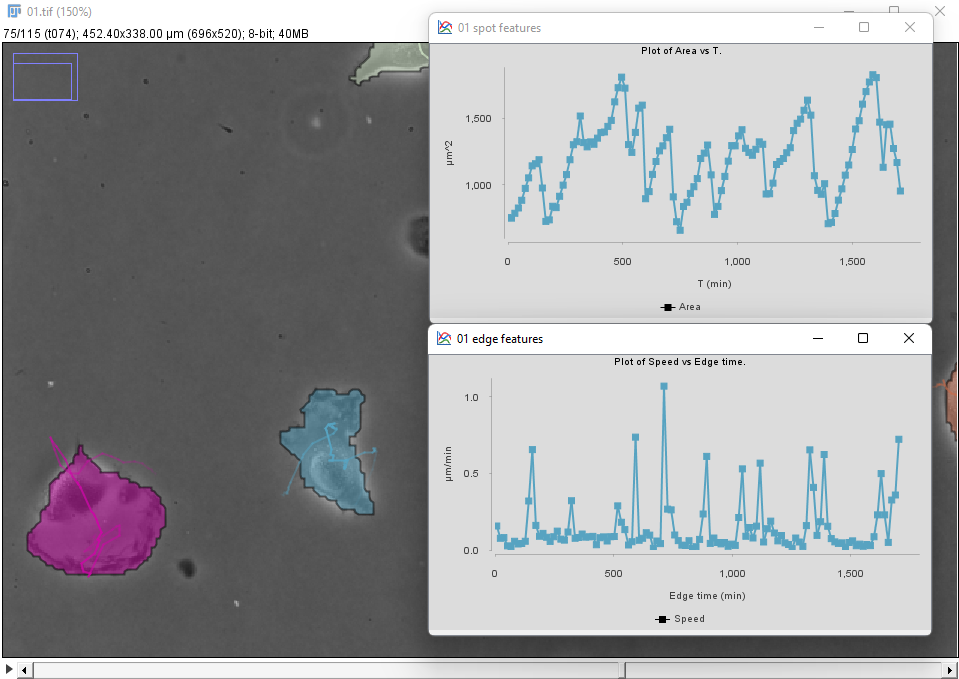
We see that brisk changes in area, corresponding to retraction events, correlate with peaks in velocity.
To generate these plots first select the cell of interest by clicking inside it in the image. In the Plot features panel, select first the Spots tab and choose T as a feature for the X axis, and Area for the Y axis. There are 3 radio buttons that allow selecting what objects will be used to plot features. In our case we want to select Tracks of selection to have the data from only the cell we selected. Click the Plot features button to generate a first graph.
The velocity is defined for links (edge between two detection across time), so click on the Links tab, and choose Edge time for X and Speed for Y. Click the Plot features button to generate the second graph.
The same metrics are different for the cell on the right:
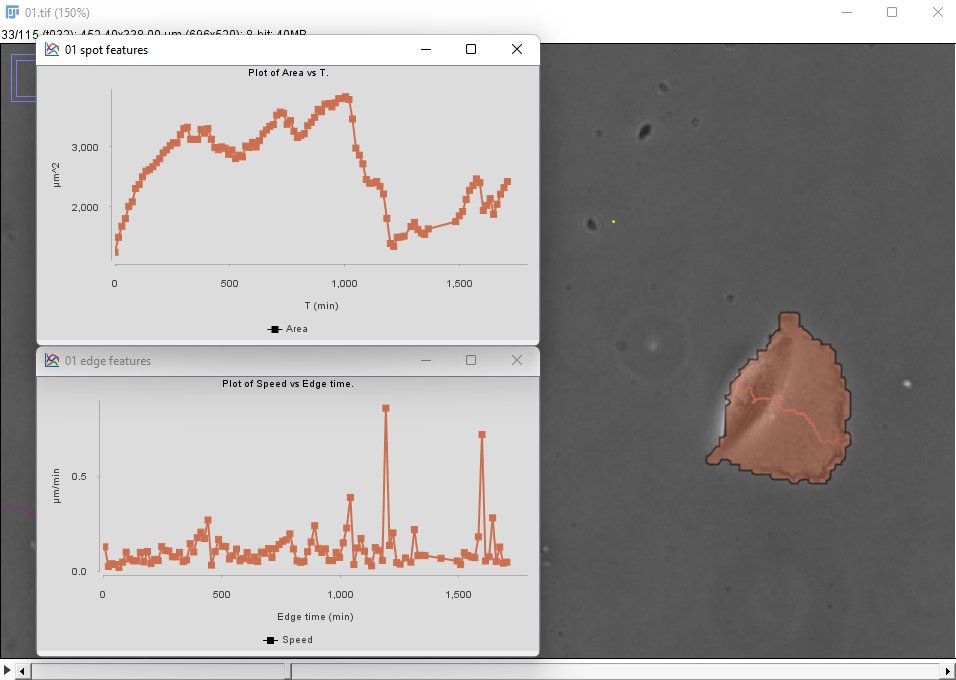
There seems to be a peak in velocity at late times along with a decrease in area, but this might be due to the cell crossing the right border of the image. We can prune these incorrect data points by filtering out the cells that touch the borders of the image.
To do this, navigate back in TrackMate to the Spot filter panel. We will add a filter on the cell position to hide the detections too close to the border. Let’s add a filter that keeps cells which center is below 420 µm:
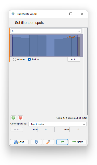
Then proceed as before for the tracking step and the plot generation. The area and velocity plots for the filtered cell track does not show the peak in velocity we had without filtering.
Additional informations
Tip: Passing RGB images to TrackMate for Cellpose
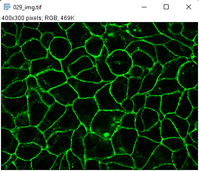
On the Cellpose website you can find a collection of test images to test with cellpose. They will work with the TrackMate integration as well, but they are RGB images. TrackMate does not support RGB images. So we give here a short optional procedure on how to feed RGB images to TrackMate and have them still segmented by cellpose as expected. Again, if you don’t have RGB images as input, you can skip this section.
cellpose can and does work with RGB images. They are single-channel but encode red, green and blue components of each pixel in one value, effectively behaving as a 3-channels 8-bit image. However, TrackMate cannot deal with RGB images. If you launch TrackMate with an RGB image you will receive an error message. The workaround is to convert them to a proper 3-channels 8-bit image before running TrackMate. cellpose will be able to run with them anyway. Here is how to do it.
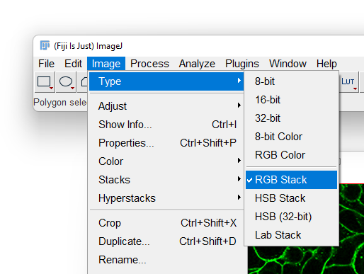
- With the RGB image opened, go to the Image › Type menu and select
RGB Stack. This will convert the 1-channel RGB image in a 3-channels 8-bit image.
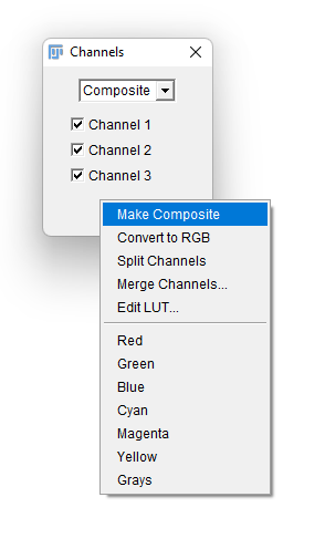
- Most likely Fiji will display only one of the 3 channels in grayscale. To overlay again the 3 channels in a composite image, first display the Channels tool by selecting the Image › Color › Channels Tool… menu item.
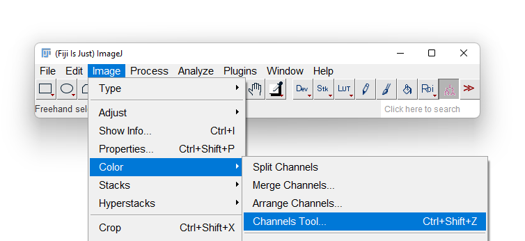
- A new floating window title Channels appears. Click on the
More »button to bring an additional menu, and select theMake Compositeitem. You image should be now properly displayed, but made of 3 independent components. This way you can run it through TrackMate and still have it properly segmented by its cellpose integration.
Installing Cellpose
This is the recommended way to install Python tools to be used with TrackMate.
This detector supports Cellpose 3 in TrackMate. It is great, simple to install, and has GPU acceleration on all modern platforms. There is a separate detector for Cellpose SAM, linked above.
You need to have conda (or mamba) installed on your system. Any flavor (Anaconda, miniconda, miniforge, mamba, micromamba, … ) works, but if you have to install one, we recommend miniforge.
Once it is done, go to the cellpose GitHub webpage and follow the installation procedures. We copy and adapt these installation instructions below. In a terminal where conda is usable, type the following (assuming you run zsh):
conda create --name cellpose-3 python=3.10
conda activate cellpose-3
pip install 'cellpose[gui]==3.1.1.2'
cellpose --version
cellpose version: 	3.1.1.2
platform:       	darwin
python version: 	3.10.18
torch version:  	2.7.1
This will install the version 3 of cellpose. As mid 2025, GPU-acceleration is used even on Mac, as you can attest in the log when running cellpose:
2025-07-11 11:13:53,625 [INFO] ** TORCH MPS version installed and working. **
2025-07-11 11:13:53,625 [INFO] >>>> using GPU (MPS)
On Windows, we noticed that it is not enough to get GPU acceleration even if you have a NVIDIA card. You need to reinstall torch with GPU CUDA support, as follow:
- Remove the current version of torch
pip uninstall torch - Reinstall torch with GPU support. Follows the instructions here.
In August 2025, this amounts to:
pip3 install torch torchvision --index-url https://download.pytorch.org/whl/cu126
Then:
cellpose --version
cellpose version:       3.1.1.2
platform:               win32
python version:         3.10.18
torch version:          2.8.0+cu126
Jean-Yves Tinevez - December 2025