Brightness and Contrast
 Brightness is the visual perception of reflected light. Increased brightness refers to an image’s increased luminance.
Contrast is the separation of the lightest and darkest parts of an image. An increase in contrast will darken shadows and lighten highlights. Increasing contrast is generally used to make objects in an image more distinguishable.
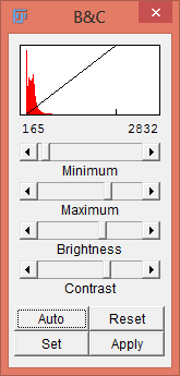
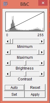
Adjust the brightness and contrast with Image › Adjust › Brightness/Contrast… to make visualization of the image easier.
Press the Auto button to apply an intelligent contrast stretch to the the image display. Brightness and contrast is adjusted by taking into account the image’s histogram. If pressed repeatedly, the button increases the percentage of saturated pixels.
The Reset button makes the “maximum” 0 and the “minimum” 255 in 8-bit images and the “maximum” and “minimum” equal to the smallest and largest pixel values in the image’s histogram for 16-bit images.
If the Auto button does not produce a desirable result, use the region-of-interest (ROI) tool to select part of the cell and some background, then hit the Auto button again. The stretch will then be based on the intensities of the ROI.
Pressing the Apply button permanently changes the actual grey values of the image. If just analyzing image intensity do not press this button.
If you prefer the image to be displayed as “black on white” rather than “white on black”, then use the “inverted” command: Image › Lookup Tables › Invert LUT. The command Edit › Invert inverts the pixel values themselves permanently.
Getting intensity values from single ROI
If working with a stack, the ROI selected can be analyzed with the command: Image › Stacks › Plot Z Axis Profile. This generates a single column of numbers - one slice intensity per row.
The top 6 rows of the column are details of the ROI. This makes sure the same ROI is not analyzed twice and allows you to save any interesting ROIs. The details are comprised of area, x-coordinate, y-coordinate, AR, roundness, and solidity of the ROI. If the ROI is a polyline>freehand ROI rather than a square>oval, it acts as if the ROI is an oval>square. The (oval) ROI can be restored by entering the details prompted by the Edit › Selection › Restore Selection (hotkey: ⌃ Ctrl + ⇧ Shift + E) command.
The results are displayed in a plot-window with the ROI details in the plot window title. The plot contains the buttons List, Save, Copy. The Copy button puts the data in the clipboard so it can be pasted into an Excel sheet. The settings for the copy button can be found under Edit › Options › Profile Plot Options. Recommended settings include: Do not save x-values (prevents slice number data being pasted into Excel) and Autoclose so that you don’t have to close the analyzed plot each time.
Dynamic intensity vs Time analysis
The plugin Plot Z Axis Profile (this is the Z Profiler from Kevin (Gali) Baler (gliblr at yahoo.com) and Wayne Rasband simply renamed) will monitor the intensity of a moving ROI using a particle tracking tool. This tool can be either manual or automatic. Use the Image › Stacks › Plot Z Axis Profile command.
Getting intensity values from multiple ROIs
You can analyze multiple ROIs at once with Bob Dougherty’s Multi Measure plugin. The native “ROI manager” function does a similar job except doesn’t generate the results in sorted columns. Check Bob’s website for updates.
The Multi Measure plugin that comes with the installation is v3.2.
- Open confocal-series and remove the background (See Background correction)
- Generate a reference stack for the addition of ROIs. Use the Image › Stacks › Z-project function and select the Average.
- Rename this image something memorable.
- Open the ROI Manager plugin (Analyze › Tools › Roi Manager or toolbar icon).
- Select ROIs and “Add” to the ROI manager. Click the “Show All” button to help avoid analyzing the same cell twice.
- After selecting ROIs to be analyzed in the reference image, you can draw them to the reference image by clicking the “More>>” button and selecting Draw. Save the reference image to the experiment’s data folder and then click on the stack to be analyzed.
- Click the “More>>” button in the ROI manager and select the Multi Measure button to measure all the ROIs. Click Ok. This will put values from each slice in to a single row with multiple columns per slice. Clicking on “Measure all 50 slices” will put all values from all slices and each ROI in a single column.
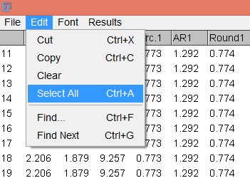
- Go to the Results window and select the menu item Edit › Select All…. Then Edit › Copy.
- Go to Excel and paste in the data. Check that everything was pasted in correctly
10. To copy ROI coordinates into the Excel spreadsheet, there needs to be an empty row above the intensity data. Use the Multi Measure dialog and click the Copy list button.
14. In Excel, click the empty cell above the first data column and paste in the ROI coordinates. Save the ROIs with the Multi Measure button Save. Put them in the experimental data folder. The ROIs can be opened later either individually with the button Open or all at once with the button Open All.
Oval and rectangular ROIs can be restored individually from x, y, l, h values with the Plugins › ROI › Specify ROI… command.
Ratio Analysis
Ratiometric imaging compares the recordings of two different signals to see if there are any similarities between them. It is done by dividing one channel by another channel to produce a third ratiometric channel. This technique is useful because it corrects for dye leakage, unequal dye loading, and photo-bleaching. An example application would be measuring intracellular ion, pH, and voltage dynamics in real time.
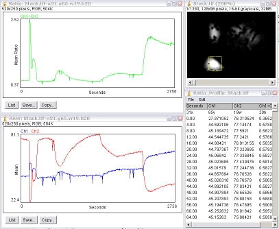
Background subtraction is needed before analysis of dual-channel ratio images. See also the background correction section. The Ratio_Profiler plugin will perform ratiometric analysis of a single ROI on a dual-channel interleaved stack. The odd-slices are channel 1 images and the even slices are channel 2 images. If your two channels are opened as separate stacks, such as Zeiss, the two channels can be interleaved (mixed together by alternating between them) with the menu command Plugins › Stacks - Shuffling › Stack Interleaver.
The plugin will generate a green-plot of the ratio values. Ch1÷Ch2 is the default and you can get Ch2÷Ch1 if the plugin is run with the ⌥ Alt key down. It will also generate a second plot of the intensities of the individual channels, Ch1 and Ch2, as well as a results table.
The first row of the results table contains values for the x, y, width and height of the ROI.
From the second row downward, the first column is the time (slice number), the second column is the Ch1 mean intensity, and the third channel is the Ch2 mean intensity and the ratio value. The stack must have its frame interval calibrated in order for the “Time” value to be in seconds. Otherwise, it is “Slices”. The frame interval can be set for the stack via the menu command Image › Properties.
This table can be copied to the clipboard and pasted elsewhere with the Edit › Copy All menu command.
Ratio Analysis Using ROI manager
1.Subtract the background from the image.
2. Open ROI manager (Analyze › Tools › ROI manager…) and click the “Show All” button.
3. Select the cells to be analyzed and add them to the ROI manager (“Add” button or keyboard T key).
4. Run the plugin.
The results window contains the mean of ch1 and ch2 and their ratio. Each row is a timepoint (slice). The first row contains the ROI details.
To generate a reference image:
- Flatten the stack with the menu command (Image › Stacks › Z-project with “Projection type: Maximum”),
- Adjust the brightness and contrast if necessary.
- Select the new image and click the “More” button in the ROI manager. After that select “Label”.
Obtaining timestamp data
Zeiss LSM
The LSM Toolbox is a project aiming at the integration of common useful functions around the Zeiss LSM file format, that should enhance usability of confocal LSM files kept in their native format, thus preserving all available metadata.
In Fiji, corresponding commands are: File › Import › Show LSMToolbox which displays the toolbox, from which all commands can be called and Help › About Plugins › LSMToolbox… which displays information about the plugin.
Biorad
This reading can be found by using the menu command Image › Show Info…. Scroll down to get the time each slice was acquired. Select this time, copy it into Excel, and find the time number obtained by using the Excel menu command Edit › Replace. This will leave only the time data. The “elapsed” time can then be calculated by subtracting row 1 from all subsequent rows.
Pseudo-linescan
Linescanning involves acquiring a single line, one pixel in width, from a common confocal microscope instead of a standard 2D image. This is usually a faster way to take an image. All the single pixel-wide images are then stacked to recreate the 2D image.
A pseudo-linescan generation of a 3-D (x, y, t) image. It is useful for displaying 3-D data in 2 dimensions.
A line of interest is drawn followed by the command: Image › Stacks › Reslice or with the keyboard button /. It will ask you for the line width that you wish to be averaged. It will generate a pseudo-linescan “stack” with each slice representing the pseudo-linescan of a single-pixel wide line along the line of interest. Average the pseudo-linescan “stack” by selecting Image › Stacks › Z-Project… and use the Average command. A poly-line can be utilized, but this will only generate a single pixel slice.
Fiji’s default settings assume that stacks are z-series rather than t-series. This means that many functions related to the third-dimension of an image stack are referred to with a z-. Just keep this in mind.
FRAP (Fluorescence Recovery After Photobleaching) Analysis
The FRAP profiler plugin will analyze the intensity of a bleached ROI over time and normalize it against the intensity of the whole cell. After that it will find the minimum intensity in the bleached ROI and fit the recovery with this point in mind.
To use:
- Open the ROI manager.
- Draw around the bleached ROI and add it to the ROI manager.
- Draw around the whole cell and add that to the ROI manager. The normalization corrects for the bleaching that occurs during image acquisition and assumes the whole cell is in the field of view. The plugin assumes the larger of the two ROIs in the ROI manager is the whole cell ROI and that the smaller ROI is the bleached part.
- Run the FRAP profiler plugin.
- The plugin will return the intensity vs time plot, the normalized intensity vs time plot of the bleached area, and the curve fit.
Non-linear contrast stretching
Equalization
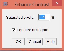
You can have more control over brightness and contrast adjustments with the Process › Enhance contrast menu command. With a stack, it analyzes the each slice’s histogram to make the adjustment.
The Equalize contrast command applies a non-linear stretch of the histogram based on the square root of its intensity.
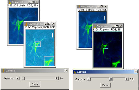
Gamma
Gamma performs a non-linear histogram adjustment. Faint objects become more intense while bright objects do not (gamma <1). Also, medium-intensity objects become fainter while bright objects do not (gamma > 1). The intensity of each pixel is “raised to the power” of the gamma value and then scaled to 8-bits or the min and max of 16-bit images.
For 8 bit images; New intensity = 255 × [(old intensity÷255) gamma]
Gamma can be adjusted via the Process › Math › Gamma command. It will allow you to adjust the gamma with the scroll bar. Click on Ok when you are finished. You can use the Scroll-bar to determine the desired gamma value on one slice of your stack. There is also an option to preview the results.
Filtering
See the online reference for an explanation of digital filters and how they work.
Filters can be found using the menu command Process › Filters….
Mean filter: the pixel is replaced with the average of itself and its neighbors within the specified radius. The menu item Process › Smooth is a 3×3 mean filter.
Gaussian filter: This is similar to a smoothing filter but instead replaces the pixel value with a value proportional to a normal distribution of its neighbors.
Median filter: The pixel value is replaced with the median of itself and its adjacent neighbors. This removes noise and preserves boundaries better than simple average filtering. The menu item Process › Noise › Despeckle is a 3×3 median filter.
Convolve filter: This allows two arrays of numbers to be multiplied together. The arrays can be different sizes but must be of the same dimension. In image analysis this process is generally used to produce an output image where the pixel values are linear combinations of certain input values.
Minimum: This filter, also known as an erosion filter, is a morphological filter that considers the neighborhood around each pixel and, from this list of neighbors, determines the minimum value. Each pixel in the image is then replaced with the resulting value generated by each neighborhood.
Maximum: This filter, also known as a dilation filter, is a morphological filter that considers the neighborhood around each pixel and, from this list of neighbors, determines the maximum value. Each pixel in the image is then replaced with the resulting value generated by each neighborhood.
Kalman filter: This filter, also known as the Linear Quadratic Estimation, recursively operates on noisy inputs to compute a statistically optimal estimate of the underlying system state.
Background correction
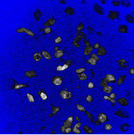
Background correction can be done in multiple ways. A simple method is to use the Image › Lookup Tables › HiLo LUT to display zero values as blue and white values (pixel value 255) as red.
With a background that is relatively even across the image, remove it with the Brightness/Contrast command by slowly raising the Minimum value until most of the background is displayed blue. Press the Apply button to make a permanent change.
Rolling-Ball background correction
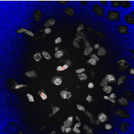
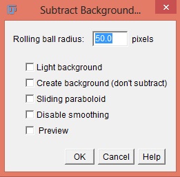
To fix an uneven background use the menu command Process › Subtract background. This will use a rolling ball algorithm on the uneven background. The radius should be set to at least the size of the largest object that is not part of the background. It can also be used to remove background from gels where the background is white. Running the command several times may produce better results. The user can choose whether or not to have a light background, create a background with no subtraction, have a sliding paraboloid, disable smoothing, or preview the results. The default value for the rolling ball radius is 50 pixels.
| RAW | Process › Subtract Background… | |
|---|---|---|
 |
 |
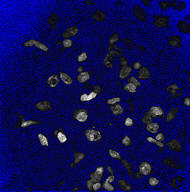 |
Once the background has been evened, final adjustments can be made with the Brightness/Contrast control.
 |
 |
 |
ROI background correction
The rolling-ball algorithm takes a lot of time. To speed up the process with an image that has a more even background, select a region of interest from the background and subtract the mean value of this area for each slice from each slice. Use the selection tools to select an area of background and run the menu command Process › Subtract Background. This macro will subtract the mean of the ROI from the image plus an additional value equal to the standard deviation of the ROI multiplied by the scaling factor you enter. The default for this is 3.
This macro, because it also works with stacks, can be used on time-courses with varying backgrounds.
| Before correction | Background intensity over time | After ROI_BG_Correction |
|---|---|---|
 |
 |
 |
Flat-field correction
Proper correction
Use this technique on brightfield images. You can correct uneven illumination or dirt/dust on lenses by acquiring a “flat-field” reference image with the same intensity illumination as the experiment. The flat field image should be as close as possible to a field of view of the cover slip without any cells/debris. This is often not possible with the experimental cover slip, so a fresh cover slip may be used with approximately the same amount of buffer as the experiment.
| RAW | Flat-field | Processed |
- Open both the experimental image and the flat-field image.
- Click the Select all button on the flat-field image and measure the average intensity. This value, the k1 value, will appear in the results window.
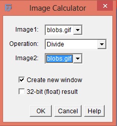
- Use the Image Calculator plus plugin (Analyze › Tools › Calculator plus).
- i1 = experimental image; i2 = flat-field image; k1 = mean flat-field intensity; k2 = 0. Select the “Divide” operation.
This can also be done using the Process › Image Calculatorfunction with the 32-bit Result option checked. Then adjust the brightness and contrast and convert the image to 8-bit.
Pseudo-correction
Sometimes it is not possible to obtain a flat-field reference image. It is still possible to correct for illumination intensity, though not small defects like dust, by making a “pseudo-flat field” image by performing a large-kernel filter on the image to be corrected. For those working with DIC images, this is particularly useful because they generally have an intrinsic, and distracting, gradient in illumination.
This can be accomplished simply by subtracting the Gaussian-blurred image version of the image.
This can also be used with stacks for brightfield time-courses that vary in intensity with time. Doing this with stacks can be time consuming.
The first RAW image (top) is pseudo-flat field corrected. Here the pseudo-flat field corrects for the uneven illumination, but does not correct for the dust specks. Look at this compared to the result of a proper flat-field correction above.
FFT background correction
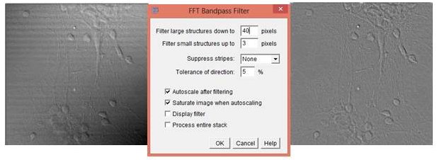
You can correct for uneven illumination and horizontal “scan lines” in transmitted light images acquired using confocal microscopes by using the native FFT bandpass function (Process › FFT › Bandpass Filter…).
You can experiment with the settings to optimize the filtering and also choose to filter structures down to a certain number of pixels. The default value is 40 pixels. You can filter small structures up to a certain value. The default value is 3 pixels. The user can choose from a drop down menu whether to suppress stripes with None, Horizontal, or Vertical. The tolerance of direction can be chosen. The default is 5%. Finally, the user can choose whether to allow autoscale after filtering, saturation of the image when autoscaling, whether or not to display the filter, and whether or not to process an entire stack.
Masking unwanted regions
Simple masking
Use one of the ROI tools to draw around the area of interest and then select: Edit › Clear outside. This will change the area outside the selected region to the background value.
Complex masking
More sophisticated masking can be done by thresholding the image and subtracting the new binary image from the original image.
- Duplicate the image, or, if it’s a stack, generate an average projection of a few frames.
- Threshold this image with the menu command Image › Adjust › Threshold.
- Hit the Auto button and adjust the sliders until all the cells are highlighted red.
- Click Apply Check the following box: black foreground, white background. You should now have a white and black image with your cells black and background white. If you have white cells and black background, invert the image with Edit › Invert.
- This can be smoothed with the command Process › Smooth and the black area enlarged slightly with Process › Binary › Dilate to give a better mask.
- Using the regular Image calculator Process › Image calculator subtract this black and white “mask” image from your original image or stack.