Getting started with TrackMate

Introduction

This tutorial is the starting point for TrackMate users. It explains how it works by walking you through a simple case, using an easy image.

The TrackMate plugin provides a way to semi-automatically segment spots or roughly spherical objects from a 2D or 3D image, and track them over time. It follows the classical scheme, where the segmentation step and the particle-linking steps are separated. Therefore each step is handled in the user interface by a specific panel, and you will go back in forth through them. Also, TrackMate has a fishing net with small holes: it will find as much spots as it can, even the ones you are not interested. So there is a step to filter them out before tracking. In these views, TrackMate resembles a bit to the Spot Segmentation Wizard of Imaris™.

The test image

The test image we will use for this tutorial has now a link in Fiji. You can find it in File › Open Samples › Tracks for TrackMate (807K), at the bottom of the list.

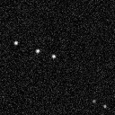
This is 128x128 stack of 50 frames, uncalibrated. It is noisy, but is still a very easy use case: there is at most 4 spots per frame, they are well separated, they are about the same size and the background is uniform. It is such an ideal case that you would not need TrackMate to deal with it. But for this first tutorial, it will help us getting through TrackMate without being bothered by difficulties.

Also, if you look carefully, you will see that there are two splitting events - where a spot seems to divide in two spots in the next frame, one merging event - the opposite, and a gap closing event - where a spot disappear for one frame then reappear a bit further. TrackMate is made to handle these events, and we will see how.

Starting TrackMate

With this image selected, launch TrackMate from the menu Plugins › Tracking › TrackMate or from the search bar. The TrackMate GUI appears next to the image, displaying the starting dialog panel.

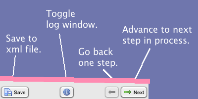
But first, just a few words about its look. The user interface is a single frame - that can be resized - divided in a main panel, that displays context-dependent dialogs, and a permanent bottom panel containing the four main buttons depicted on the right.

The Next button allows to step through the tracking process. It might be disabled depending on the current panel content. For instance, if you do not select a valid image in the first panel, it will be disabled. The Previous button steps back in the process, without executing actions. For instance, if you go back on the segmentation panel, segmentation will not be re-executed.

The Save button creates a XML file that contains all of the data you generated at the moment you click it. Since you can save at any time, the resulting file might miss tracks, spots, etc… You can load the saved file using the menu item Plugins › Tracking › Load a TrackMate file. It will restore the session just where you saved it.

Now is a good time to speak strategy when it comes to saving/restoring. You can save at anytime in TrackMate. If you save just before the tracking process, you will be taken there with the data you generated so far upon loading. TrackMate saves a link to the image file (as an absolute file path) but not the image itself. When loading a TrackMate file, it tries first to retrieve and open this file in ImageJ. So it is a good idea to pre-process, crop, edit metadata and massage the target image first in Fiji, then save it as a .tif, then launch TrackMate. Particularly if you deal with a multi-series file, such as Leica .lif files.

The advantage of this approach is that you load in TrackMate, and everything you need will be loaded and displayed. However, if you need to change the target file or if it cannot be retrieved, you will have to open the TrackMate XML file and edit its 4th line.

The start panel

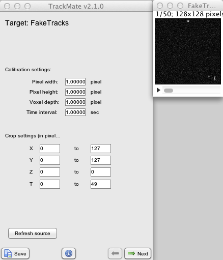
This first panel allows you to check the spatial and temporal calibration of your data. It is very important to get it right, since everything afterwards will be based on physical units and not in pixel units (for instance μm and minutes, and not pixels and frames). In our case, that does not matter actually, since our test image has a dummy calibration (1 pixel = 1 pixel).

What is critical is also to check the dimensionality of the image. In our case, we have a 2D time-lapse of 50 frames. If metadata are not present or cannot be read, ImageJ tends to assume that stack always are Z-stack on a single time-point.

If the calibration or dimensionality of your data is not right, I recommend changing it in the image metadata itself, using Image › Properties (⌃ Ctrl + ⇧ Shift + P). The press the ‘Refresh source’ button on the TrackMate start panel to grab changes.

You can also define a sub-region for processing: if you are only interested in finding spots in a defined region of the image, you can use any of the ROI tools of ImageJ to draw a closed area on the image. Once you are happy with it, press the Refresh source button on the panel to pass it to TrackMate. You should see that the X Y start and end values change to reflect the bounding box of the ROI you defined. The ROI needs not to be a square. It can be any closed shape.

If you want to define the min and max Z and/ or T, you have to edit manually the fields on the panel.

Defining a smaller area to analyze can be very beneficial to test and inspect for correct parameters, particularly for the segmentation step. In this tutorial, the image is so small and parse that we need not worrying about it. Press the Next button to step forward.

Choosing a detector

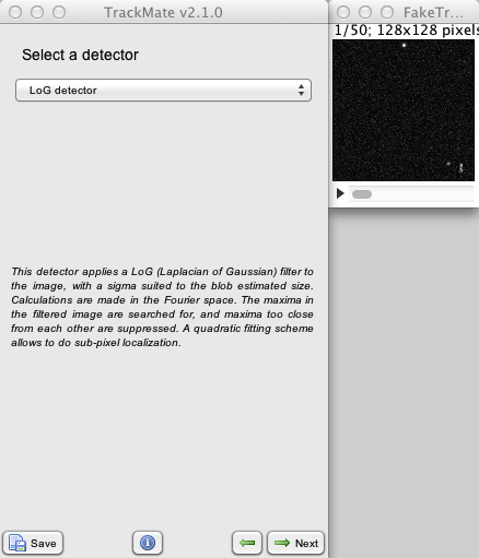
You are now offered to choose a detection algorithm (“detector”) amongst the currently implemented ones.

The choice is actually quite limited. Apart from the Manual annotation, you will find 3 detectors, but they are all based on LoG (Laplacian of Gaussian) segmentation. They are described in detail elsewhere, but here is what you need to know.

• The LoG detector applies a plain LoG segmentation on the image. All calculations are made in the Fourier space, which makes it optimal for intermediate spot sizes, between ≈5 and ≈20 pixels in diameter.
• The DoG detector uses the difference of Gaussians approach to approximate a LoG filter by the difference of 2 Gaussians. Calculations are made in the direct space, and it is optimal for small spot sizes, below ≈5 pixels.
• The Downsample LoG detector uses the LoG detector, but downsizes the image by an integer factor before filtering. This makes it optimal for large spot sizes, above ≈20 pixels in diameter, at the cost of localization precision.

In our case, let us just use the Dog detector.

The detector configuration panel

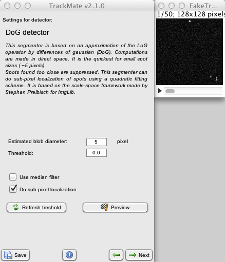
The LoG-based detectors fortunately demand very few parameters to tune them. The only really important one is the Estimated blob diameter’. Just enter the approximate size of the spots you are looking to tracks. Careful: you are expected to enter it in physical units. In our dummy example, there is no calibration (1 pixel = 1 pixel), so it does not appear here.

There are extra fields that you can configure also. The Threshold numerical value aims at helping dealing with situation where a gigantic number of spots can be found. Every spot with a quality value below this threshold value will not be retained, which can help saving memory. You set this field manually, and check how it fares with the Preview button button.

You can check Use median filter: this will apply a 3x3 median filter prior to any processing. This can help dealing with images that have a marked salt & pepper noise which generates spurious spots.

We hope that TrackMate will be used in experiments requiring Sub-pixel localization, such as following motor proteins in biophysical experiments, so we added schemes to achieve this. The one currently implemented uses a quadratic fitting scheme (made by Stephan Saalfeld and Stephan Preibisch) based on David Lowe SIFT work¹. It has the advantage of being very quick, compared to the segmentation time itself.

Finally, there is a Preview button that allows to quickly check your parameters on the current data. After some computations, you can check the results overlaid on the image. Most likely, you will see plenty of spurious spots that you will be tempted to discard by adjusting the Threshold value. This is a very good approach for large problems. Here, we care little for that, just leave the threshold at 0.

The two others automated segmenters share more or less the same fields in their own configuration panel. The Downsampled LoG segmenter simply asks for an extra down-sampling integer factor.

In our case, the spots we want to track are about 5 pixels in diameter, so this is what we enter in the corresponding field. We don’t need anything else. The Sub-pixel localization option adds a very little overhead so we can leave it on.

The detection process

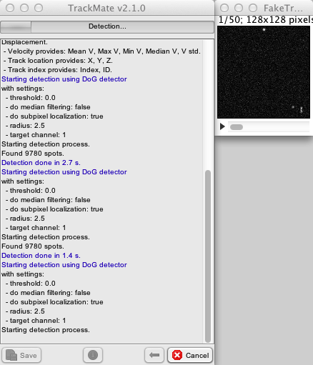
Once you are happy with the segmentation parameters, press the Next button and the segmentation will start. The TrackMate GUI displays the log panel, that you will meet several times during the process. It is basically made of a text area that recapitulates your choices and send information on the current process, and of a progress bar on top. You can copy-paste the text if you want to keep track of the process somewhere. You can even add comments as text in it: it is editable, and everything you type there is saved in the XML file, and retrieved upon loading. You can access the log panel anytime, by clicking on the log button at the bottom of the TrackMate window.

Should the process be long enough, you should be able to see that the Next button turned into a Cancel button. If you press it while the detection is running, TrackMate will finish the detection of the current frames, and stop. You could now go on with the spots it found, or go back and restart.

TrackMate takes advantage of multi-core computers, which seems to be the standard nowadays. It will segment one time-frame per core available. On computers with many cores, the progress bar will seems to move in a bulky way: if you have 16 cores, 16 time-points will be segmented at once, and it is likely that they will be finished approximately on the same time. So don’t be worried if the progress bar does not move in the beginning for large images.

On our dummy image, this is clearly something we need to worry about, and the segmentation should be over in a few seconds. Typically, this is the step that takes the longer. Once the segmentation is done, the Next button is re-enabled.

Initial spot filtering

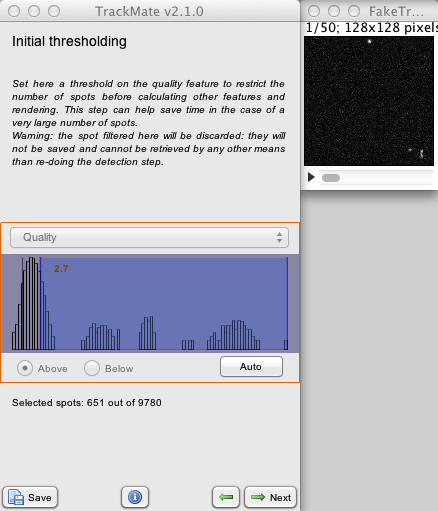
Here is a difficult step to explain, particularly because we do not need at all now. If the explanations following in this paragraph seem foggy, please feel free to press the Next button and skip to the next paragraph. This one is all related to performance, memory and disk usage in difficult cases.

TrackMate uses generic segmentation algorithms for which there is only a little number of parameters to specify. The price to pay then, is that you can get a lot of undesired spots as an outcome. And in some cases, a really large amount of those.

This is why there is spot features and feature filters. In the next steps, each spot will have a series of numerical features calculated using its location, radius and the image it is found in, such as the mean pixel intensity. You will be able to define filters on these features, to retain only the ones that are relevant to your study.

But for a very large number of spots - let’s say: more than 1 million of them - performance issues can kick in. Those millions of spots will be stored in the model, and saved in the TrackMate file, in case you want to step back and change the filters, because for instance you realized you are not happy with the end results (you can do that). Some visualization tools - the 3D displayer for instance - will generate the renderings for those millions of spots at once and hide or show them depending on the filter values, because it is too expensive to recreate the renderings while tuning the filter values.

To deal with that, we added a first filter prior to any other step, that uses the Quality value. The quality value is set by the segmenter, and is an arbitrary measure of the likelihood of each spot to be relevant. This panel collects all the quality values for all spots, and display their histogram (Y-scale is logarithmic). You can manually set a threshold on this histogram by clicking and dragging in its window. All spots with a quality value below this threshold will be discarded. That is: they will be deleted from the process, not saved in the file, they won’t be displayed, nor their features will be calculated. Which is what we want when meeting a gigantic number of spurious spots. Note that this step is irreversible: if you step back to this panel, you will see the original histogram, but beware that the spots you have discarded cannot be recovered by changing the threshold. The only way is to step back further and restart the segmentation step.

In our case, we see from the histogram that we could make sense of this step. There is a big peak at low quality (around a value of 1.2) that contains the majority of spots and is most likely represent spurious spots. So we could put the threshold around let’s say 5.5 and probably ending in having only relevant spots. But with less than 10 000 spots, we are very very far from 1 million so we need not to use this trick. Leave the threshold bar close to 0 and proceed to the next step.

Selecting a view

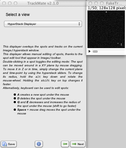
Here, you can choose between the two visualization tools that will be used to display the tracking results. The first one, HyperStack displayer, simply reuses ImageJ stack window and overlay the results non-destructively over the image. Choosing the 3D viewer will open a new 3D viewer window, import that image data in it, and will display spots as 3D spheres and tracks as 3D lines.

Honestly, choose the HyperStack displayer. Unless you have a very specific and complicated case that needs to inspect results in 3D immediately, you do not need the 3D viewer. The HyperStack displayer is simpler, lighter, allow to manually edit spots, and you will be able to launch a 3D viewer at the end of the process and still get the benefits.

When you press the Next button, two processes start:

• the features of all spots (well, those you left after the initial filtering step) are calculated;
• the displayer selected does everything it needs to prepare displaying them.

So nothing much. Let’s carry on.

Spot filtering

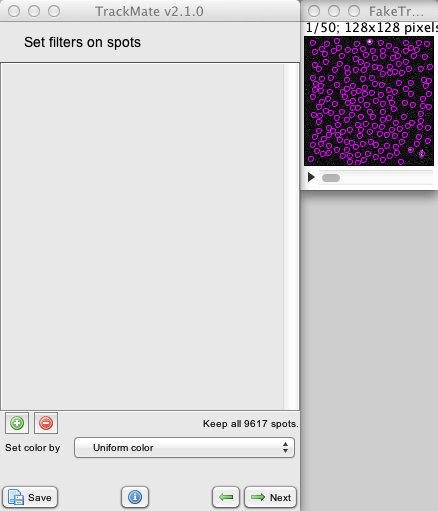
The moment this panel is shown, the spots should be displayed on the ImageJ stack. They take the shape of purple circles of diameter set previously. As promised, there are quite a lot of them, and their vast majority are irrelevant. If you did not remove the irrelevant one in the initial thresholding step, you should get an overlay that resembles the image to the right.

Trying to do particle linking on all these spots would be catastrophic, and there would be no hope to make sense of the data as it is now. This is why there is this spot filtering step, where you can use the features we just calculated to select the relevant spots only.

The spot filtering panel is divided in two. The upper part, which is empty now, contains the filter you define, in the shape of histograms. We will come back to them soon. The bottom part contains the + and minus buttons that allow to respectively add or remove a feature filter, and a combo-box to set the display color of the spots.

Let us try it to play with it to find the best feature to filter out spurious spots.

By default , when the combo-box is on Uniform color, all spots are purple. By clicking on it, you see that you can select amongst all the possible features calculated. For instance, if you select X, the spots will be colored according to their X position. A colored bar below the combo-box indicates the range the color gradient corresponds to.

X does not seem to be a good feature to select relevant spots. We know that Quality should be, by construction, but let us pick Mean intensity. By scrolling through the time slide you should be able to see that now all the spurious spots have a blue to turquoise color, whether the real one stands forward in red or yellow.

We will therefore add a filter based on this feature. Click the green + button. A small orange box should appear in the upper part, containing the histogram for a given feature. Click on the orange box combo-box to select Mean intensity. Yous should have something similar to the image below.

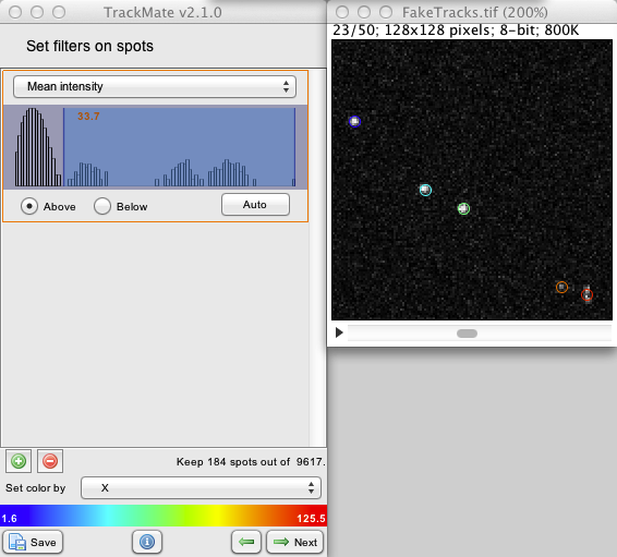
We note that the histogram has a very desirable shape: a massive peak at low intensity represent most of the spots. There are other smaller peaks at higher intensity, and fortunately, they are very well separated from the large peak.

To move the threshold, simply click and drag inside the histogram window. Notice how the overlay is updated to display only the remaining spots after filtering.

Interlude: A word on the GUI: I put some effort into having a GUI that can be navigated almost solely with the keyboard. Any of the small filter panel can be controlled with the keyboard. For instance: give the histogram the focus by either pressing the Tab key or clicking into it.

• The floating threshold value should turn from orange to dark red. You can now type a numerical value (including decimals using the dot ‘.’ as separator); wait two seconds, and the threshold value will be updated to what you just typed.
• Ot use the arrow keys: the left and right arrow keys will change the threshold value by 10%, the up and down arrow will set it to the max and min value respectively.

A filter can be set to be above or below the given threshold. You change this behavior using the radio buttons below the histogram window. In our case, we want it to be above of course. The Auto button uses Otsu’s method to determine automatically a threshold. In our case, we will put it manually around 33.

You can inspect the data by scrolling on the hyperstack window and check that only mostly good spots are retained. This is an easy image. The spots you have filtered out are not discarded; they are simply not shown and they will not be taken into account when doing particle linking. In a later stage, you can step back to this step, and retrieve the filtered out spots by removing or changing the filters.

You can stack several filters by simply clicking on the green + button. TrackMate will retain the spots that satisfy to all (logical and) the criteria set by the filters.

Press Next when you are ready to build tracks with these spots.

Selecting a simple tracker

The next panel let you choose amongst available particle-linking algorithms, or “trackers”.

The apparent profusion of choices should not disorient you, for it just that: an appearance. We chose to focus on the Linear Assignment Problem (LAP) in the framework first developed by Jaqaman et al.².

The first two LAP trackers are based on LAP, with important differences from the original paper described here . We focused on this method for it gave us a lot of flexibility and it can be configured easily to handle most cases. You can tune it to allow splitting events, where a track splits in two, for instance following a cell that encounters mitosis. Merging events are handled too in the same way, though my small culture prevents me from quoting a relevant biological case obvious as the previous one. More importantly are gap-closing events, where a spot disappear for one frame (because it moves out of focus, because segmentation fails, …) but the track manages to recuperates and connect with reappearing spots later.

These LAP algorithm exists in TrackMate in two flavors: a simple one and a not simple one. There are again the same, but the simple ones propose fewer configuration options and a thus more concise configuration panel. In short:

• The simple one only allows to deal with gap-closing events, and prevent splitting and merging events to be detected. Also, the costs to link two spots are computed solely based on their respective distance.

• The not simple one allows to detect any kind of event, so if you need to build tracks that are splitting or merging, you must go for this one. If you want to forbid the detection of gap-closing events, you want to use it as well. Also, you can alter the cost calculation to disfavor the linking of spots that have very different feature values.

There is also a 3rd tracker, the Nearest neighbor search tracker. This is the most simple tracker you can build, and it is mostly here for demonstration purposes. Each spot in one frame is linked to another one in the next frame, disregarding any other spot, thus achieving only a very local optimum. You can set a maximal linking distance to prevent the results to be totally pathological, but this is as far as it goes. It may be of use for very large and easy datasets: its memory consumption is very limited (at maximum only two frames need to be in memory) and is quick (the nearest neighbor search is performed using Kd-trees).

Then of course, there is the option to skip the automated tracking using Manual tracking.

Right now, in our first trial, let us pick the Simple fast LAP tracker.

Configuring the simple LAP tracker

As promised, there is only three configuration fields.

• The first one defines the maximal allowed linking distance. This value limits the spatial search range for candidate matching spots. If you know the maximal displacement of your object between two frame, you can put this value here. Theoretically, a too large value will demand more computation time. In our case, seeing the size of the dataset, this does not matter at all. This distance must be expressed in physical units, but again, you don’t see it there for there is no spatial calibration on our image.

• The second field defines the maximal distance for gap-closing. Two track segments will not be bridged if the last spot of the first segment is further away than the first spot of the second segment. In our dummy example stack, there is spot disappearance at the frame number 45, top left. So the spot on frame 44 and the spot on frame 46 must not be separated by more than the distance you set there to have a chance to be linked.

• The third field also deal with the detection of gap-closing events, and sets the maximal frame interval between two spots to be bridged. Careful, the time is set in frame interval, here we do not want the physical time. In our case, since the only disappearance event we have last one frame, we can simply put this value to 2 frames duration. But actually it does not matter, as you can see by experimenting.

Press Next to start the tracking computation.

Our first tracking results

You are now shown the log panel, where the tracking process is logged. Since our dataset is very small, it should complete very quickly. Press Next again to see the results. They should look like this:

Basically, the tracker held its promises: there is 6 tracks (the two immobile spots at the bottom left part of the image contributed a track each). These tracks are not branching. The red track indeed contains a gap closing event, that did not generate a track break. That would have been different if we would have used the Nearest neighbor search tracker: as it cannot deal with gap-closing events, we would have 7 tracks.

The track colors are yet meaningless; there are just used to facilitate separating different tracks visually.

Now, we would like the shape of these tracks to change. We see that the yellow track is actually branching from the blue one at frame 10. The same goes for the orange track, which branches from the green one at frame 17, and merges to the blue one at frame 27. To deal with that, we need to change of tracker. So go two steps back using the Previous button and go back to the tracker choice panel. There, select the LAP tracker and move to its configuration panel.

Configuring a not so simple tracker

Look at the configuration panel. It is quite more complex than for the simple tracker, obviously, and it is the price for flexibility. Since it is quite long, the panel has to be scrolled to its bottom to venture on all fields.

However, this apparent complexity is not that difficult to harness. If you look carefully, you will see that the main panel is made of 4 quasi-identical panel. Each one deals with one event type:

The first one deals with the frame-to-frame linking. It consists in creating small track segments by linking spots in one frame to the spots in the frame just after, not minding anything else. That is of course not enough to make us happy: there might be some spot missing, failed detection that might have caused your tracks to be broken. But let us focus on this one now.

Linking is made by minimizing a global cost (from one frame to another, yet). A short word on the linking logic: The base cost of linking a particle with another one is simply the squared distance³. Following the proposal of Jaqaman et al.², we also consider the possibility for a particle not to make any link, if is advantageous for the global cost. The sum of all costs are minimized to find to set of link for this pair of frame, and we move to the next one.

As for the simple tracker, the Max distance field helps preventing irrelevant linking to occur. Two spots separated by more than this distance will never be considered for linking. This also saves some computation time.

The Feature penalties let you tune the linking cost using some measures of spot similarity. Typically in the single particle tracking framework, you cannot rely on shape descriptors to identify a single object across multiple frames, for spots are “shapeless”: they are just described by a X, Y, Z, T position tuple.

Yet, you might know your Biology better. For instance, you might be in the case where the mean intensity of a spot is roughly conserved along time, but vary even slightly from one spot to another. Or it might be the spot diameters, or a rough elliptic shape. Feature penalties allow you to penalize links between spots that have feature values that are different. Since the case you study might be anything, you can pick any feature to build your penalties. This one of the novelties in TrackMate, already evoked in Jaqaman et al.², but extended here.

If you want to use feature penalties for frame-to-frame linking, simply press the green + button in the sub-panel. A combo-box will appear, in which you can choose the target feature. The text field ti its right allows specifying the penalty weight. Feature penalties will change the base cost. We will not go in the details here (particularly because we are not going to use feature penalties in this tutorial), but basically, two spots with different features will have a linking cost higher than if the selected features values were the same. The weight allows you to specify how much you want to penalize a specific feature difference. A weight of 10 is already very penalizing.

In our case, given the sparsity of spots, we do not need help from the features at all. Remove any penalties you might have added, using the red - button.

The three other sub-panels deal with the second pass of the linking algorithm, where you take track segments created above and relink them. This gap-closing part is already known to you, it is the same as we saw in the previous section: you have to specify a maximal distance, and a maximal frame separation. You can also specify feature penalties, like for frame-to-frame linking. They will be computed on the last spot of the first segment and the first spot of the 2nd segment you are trying to bridge.

The 3rd and 4th panels deal respectively with track splitting events and track merging events. The mechanisms at play are the same that for the gap-closings: track segments are bridge together depending on the penalties and on the max distance allowed. Track splitting and merging are only allowed from one frame to the next one.

For track splitting, the middle of a segment is offered to bridge to the start of another segment. For track merging, the end of a segment is offered to bridge to the middle of another one. A check box sets if you want to forbid or allow any of these events.

As an exercise, try to find the parameters the will fuse the central track segments in a single large track, with two splitting events and a merge event. You should obtain the track layout pictured below.

Filtering tracks

The next panel is just the equivalent of the spot filtering step we met before, but this time we use track features,. The filter principles are the same: you simply add filters, choosing a target feature, until you are happy with the remaining tracks. As for the spots, the tracks are not really deleted; they are just hidden and you can retrieve them by switching back to this panel and delete the filters.

Here, we have a total of 4 tracks. The two immobile spots of the bottom left contribute one track each, that we can barely see because they do not move much. Let us say that we want to get rid of them. There are several ways to do that, but the simple is simply to add a filter on track displacement, as picture above.

The end or so

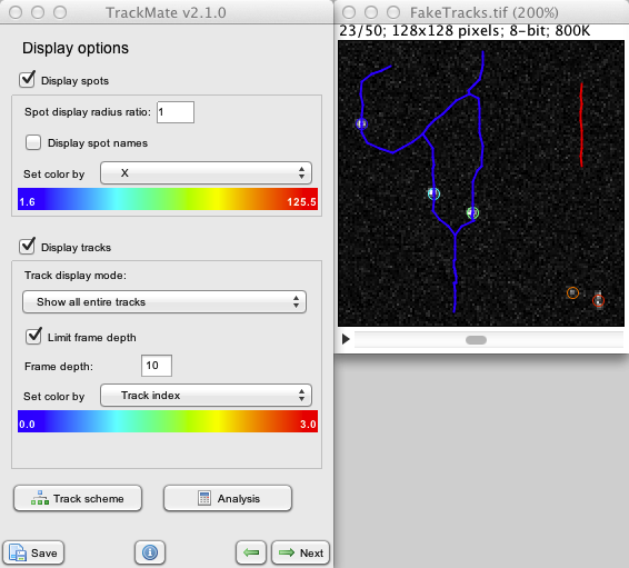
We are now close to the end of a typical workflow for a tracking problem. The panel you see now is the one that recapitulates display option. You can set spot color by feature, hide them, show their name, etc… Find out what they do, display options are pretty much self-explanatory.

The TrackScheme button launches a module that allow manually editing tracks, and performing analysis on them. It is the subject of another tutorial.

If you press Next, you will see that there is still two panels after this one. The first one allows to plot any kind of feature as a function of another one. TrackMate deals with 3 kind of features: spot, link and track feature, depending on where it makes sense to compute them. For instance, instantaneous velocity is computed over a link (between two spots linked in a track), so you will find it on the Links tab. The + and - buttons allow you add several features on the Y-axis, and they will be pooled on the same graph or not, depending on the dimensionality of the features.

The last panel is the Action chooser panel, that allows you to execute simple actions on your data, such as exporting, copying, re-calculating feature, etc…

If you are happy with the results, you can save them now. Loading the resulting file again in TrackMate will bring you to this panel, where you can inspect those results conveniently

Wrapping up

That is the end of this introductory tutorial. As you can see, it is quite long. Hopefully that does not mean that TrackMate itself is complicated. We detailed what you could do for the tracking part (the analysis and editing part is still to be seen), but if you recapitulate what we changed from the default, that was pretty simple:

• we set the segmentation diameter to 5;
• we added a spot filter on mean pixel intensity;
• we picked a not-so-simple tracker and allowed for splitting and merging;
• we added a track filter on displacement.

Now that you know how the plugin works, you should be able to reach the end result in less than 30 seconds…

Jean-Yves Tinevez (talk) 04:18, 1 August 2013 (CDT)

References