TrackMate Mask detector

This page describes a detector for TrackMate that creates objects from a black and white channel in the source image. You can add the mask as an extra channel in the source image. The objects will be built based on all the pixels have a value strictly larger than 0, which solves the issue of having a mask on 8-bit, 16-bit or 32-bit images.

Usage

There is not much to say. You need to prepare a mask for the source image you want to track using any means that work.

For 2D images, TrackMate will obtain the contour of objects, possibly simplified, from the mask. For 3D images, it will create spherical spots of an identical volume.

It is a good idea to merge this mask as an extra channel of the source image, so that you can have both the mask and the source image in TrackMate. This allows measuring numerical features on the source image based on the contours obtained with the mask.

Tutorial: C.elegans early development

The dataset

We will use a simple and short image of a C.elegans embryo. You can download the data on Zenodo:

This movie is a maximum-intensity projection (MIP) of a longer movie used initially in:

Tinevez JY, Dragavon J, Baba-Aissa L, Roux P, Perret E, Canivet A, Galy V, Shorte S. A quantitative method for measuring phototoxicity of a live cell imaging microscope. Methods Enzymol. 2012;506:291-309. doi: 10.1016/B978-0-12-391856-7.00039-1. PMID: 22341230.

This is very short movie, that stops after the 2nd cell division. We made a MIP so that this movie can be used in this tutorial.

The image

Open the image CelegansEarly_MIP.tif in Fiji.

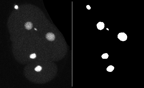
It is a 2 channels image. The first channel contains the raw image data. It shows the fluorescence collected from a C.elegans embryo, stained with eGFP-H2B, imaged on laser-scanning confocal microscope. We see the nuclei move and divide, along the with 2 smaller polar bodies.

The 2nd channel contains the segmentation results of this signal, that I obtained by applying a

• Median filter;
• Gaussian blur filter;
• Plain thresholding.

Running TrackMate

Launch TrackMate: Plugins>Tracking>TrackMate

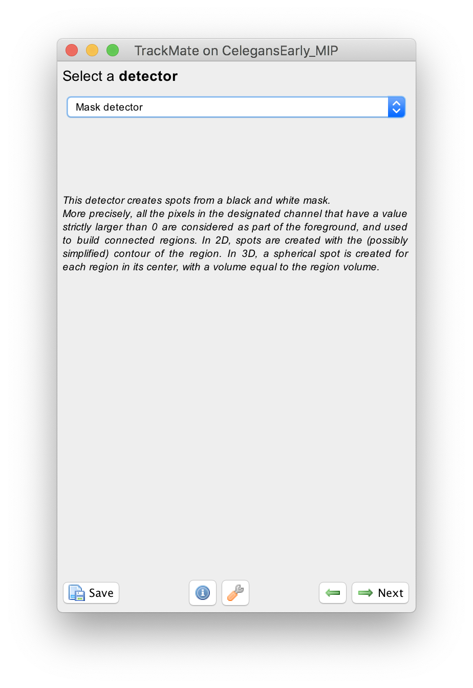
In the second panel, select the Mask detector

The configuration panel is very simple:

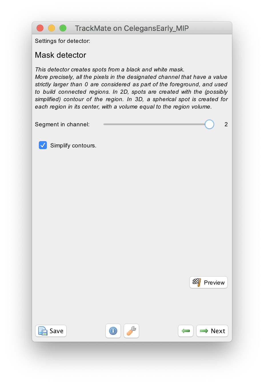
You just need to specify in what channel is the mask. In our case it is the second one.

There is a checkbox that lets you simplify contours. We suggest you leave it on by default. The details of contour simplification are explained here.

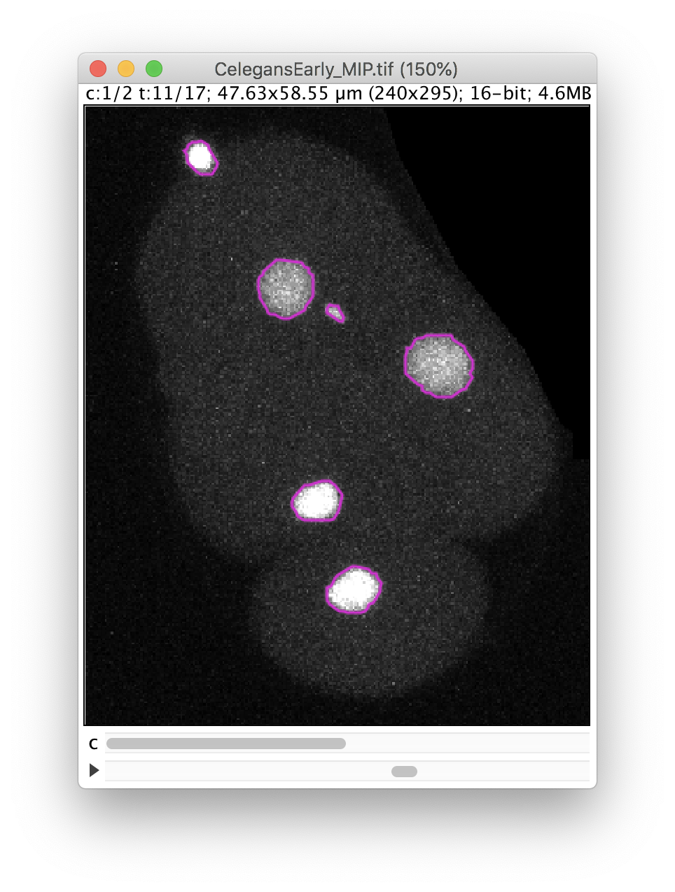
The Preview button will show the results. In frame 11 for instance, 6 objects are detected with their contour:

The click the Next button. In total 78 spots are found in this movie. You can track them with LAP tracker, enabling the detection of split events so that we can deal with the 2 cell divisions. In the end of tracking process we get this:

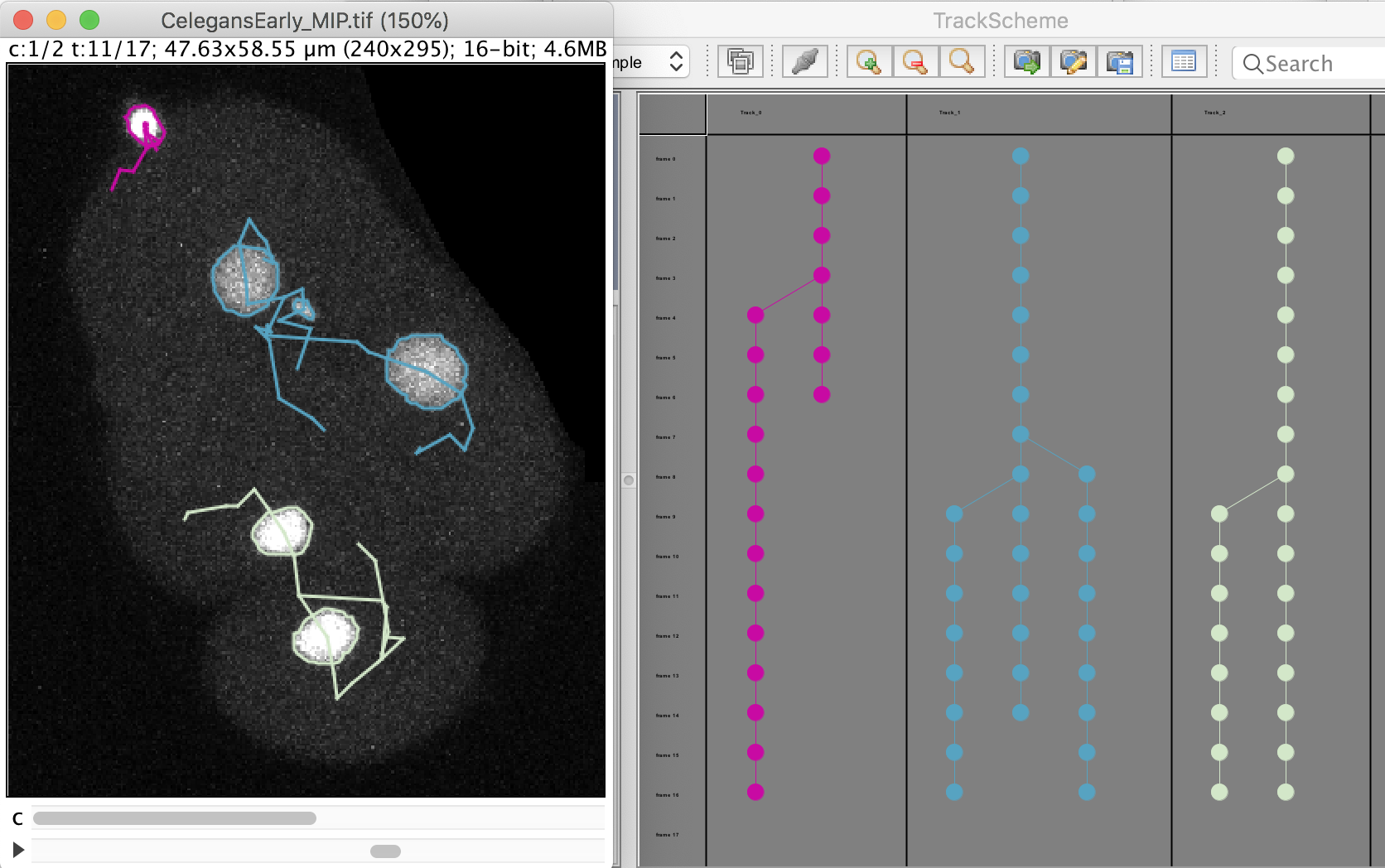
Notice that we have false divisions due to the motile polar body, that gets wrongly attached to the top cell movie. We could correct this either manually, or by filtering out the polar bodies based on their Area. We leave this correction as an exercise to the reader.

Plotting nucleus shape over time

Now that we have the cell shape and their lineage, we can follow how the shape changes as the cell divides. For instance, let’s plot the nucleus size and circularity of the bottom cell over time.

To do this, select the bottom cell by clicking in one of the spot, then moved to the Plot feature panel of the TrackMate wizard. Make sure you are in the Spots tab.

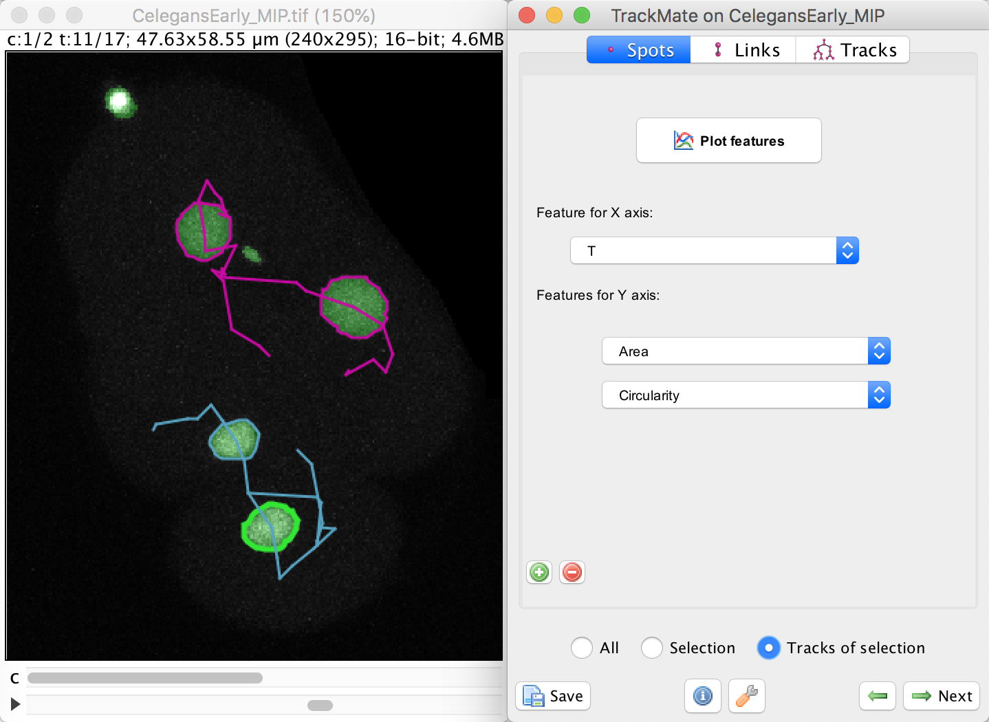
In this panel, select the Area in the Feature for Y axis first list.

Click on the green + button to add a second list of features, and select the Circularity feature. We want to plot these feature values not for a single spot, nor for the whole dataset, but just for the track of the spot we selected. To do this, select the Tracks of selection radio button at the bottom. Of course, at least one spot in the track of interest must be selected.

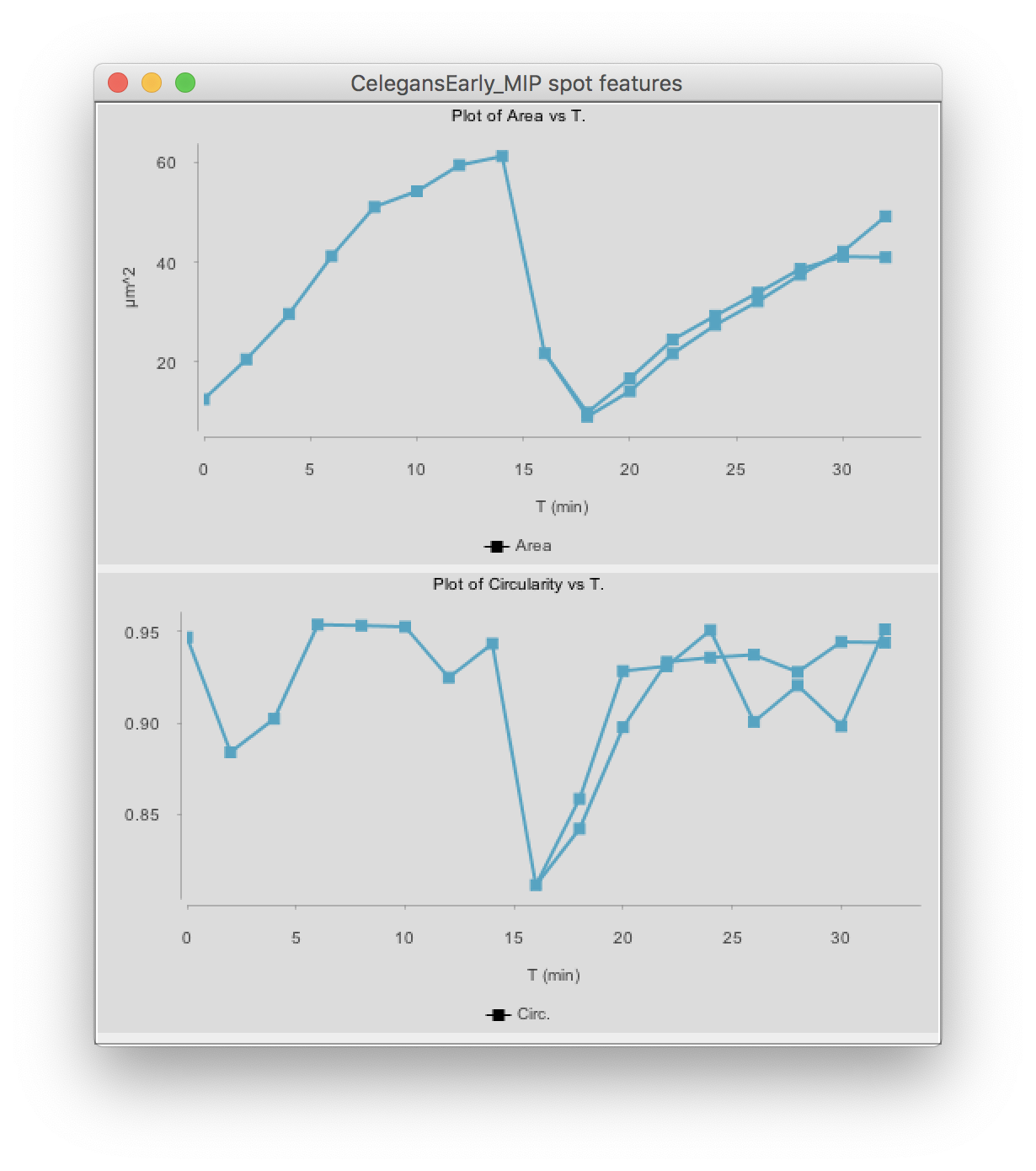
Click on the Plot features button. The two graphs appear:

(You might have to deselect the cell by clicking elsewhere, then clicking back in the graph so that it shows the same color than above.)

The top graph shows the area over time. We see that it steadily increases until the cell divides at t=15 minutes. The area sharply decreases and two cells are now plotted in the graph. Their area resume increasing, with almost identical rate.

The circularity is plotted on the second graph. It remains high almost all the time (close to 1), as the nuclei have a roughly spherical shape. When the cell divides, the nucleus takes an elongated shape, which results in a lower circularity.

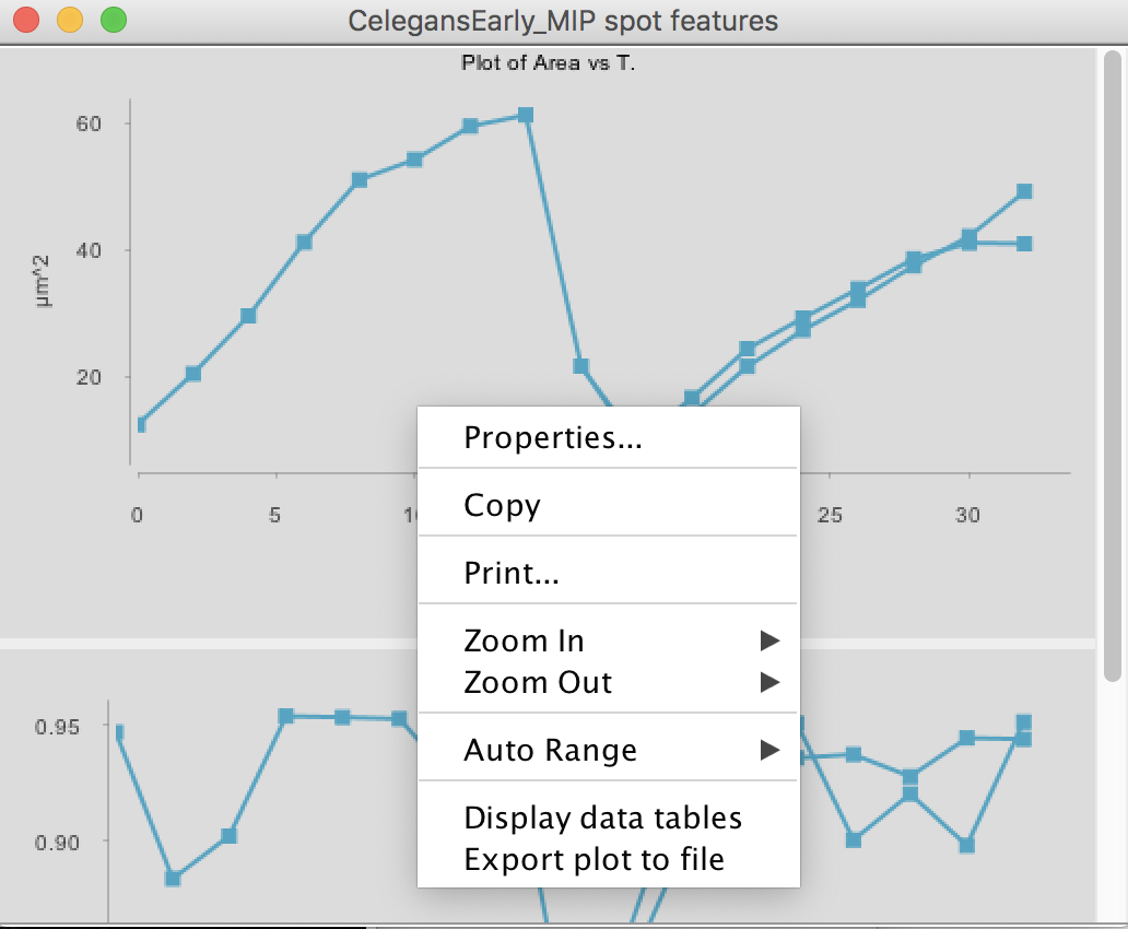
As a side note, if you right-click on any of the 2 plots, you will have this popup menu that will let you export the graph as a pdf, png or svg image, or show its data in a table that can saved to a CSV file.

Editing the mask

If we repeat the above procedure for the top cell, we have the following graphs:

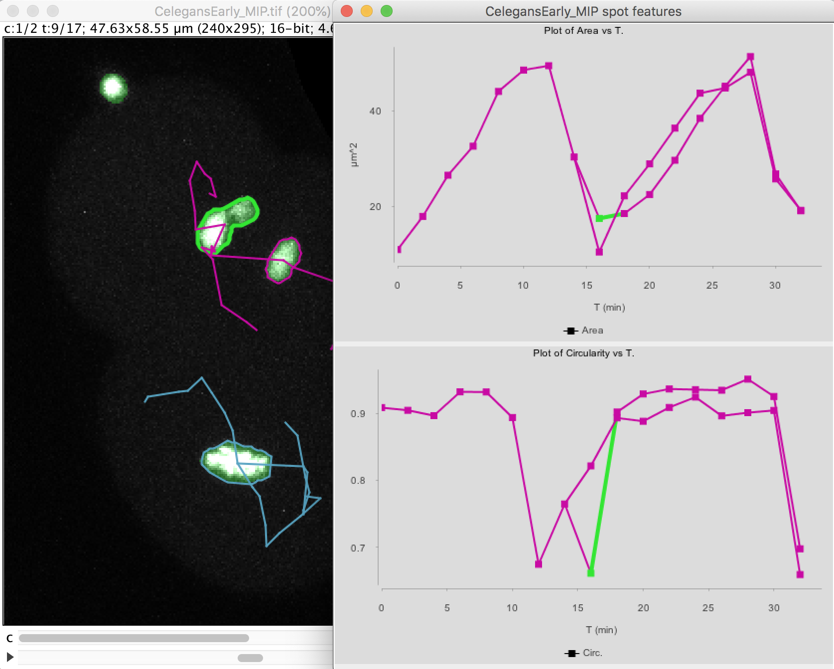
Note that at t=16 minutes, one of the daughter nuclei has a circularity that shows a sharp drop. By inspecting the image, we can see that this is caused by the object contour to be incorrect for this spot. The motile polar body went too close to the nucleus and the mask merged them together. So we end up in having an artificially elongated object, which results in a low circularity.

Right now there is no way to edit a spot contour. Here we would suggest a hack. We will directly edit the binary mask by cutting the object with Fiji tool.

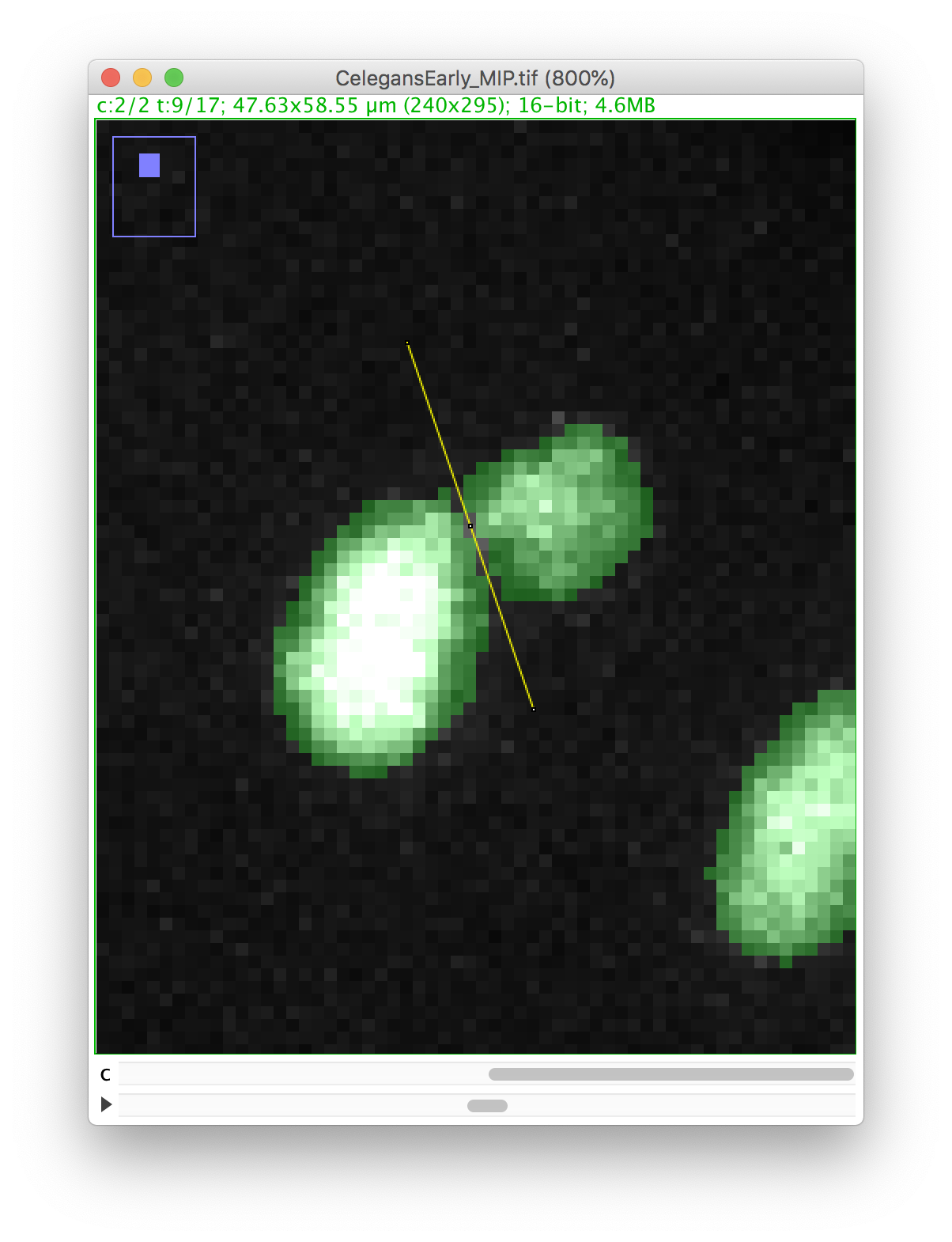
Go back to the first panel of the TrackMate wizard and in the image display, select the 9th time-point, and make the second channel active:

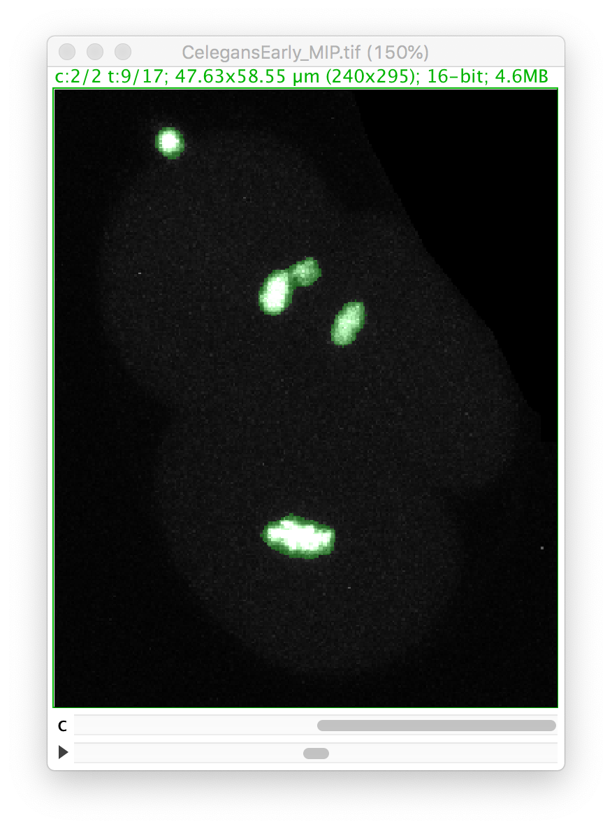
Let’s zoom on the nucleus with the defective mask.

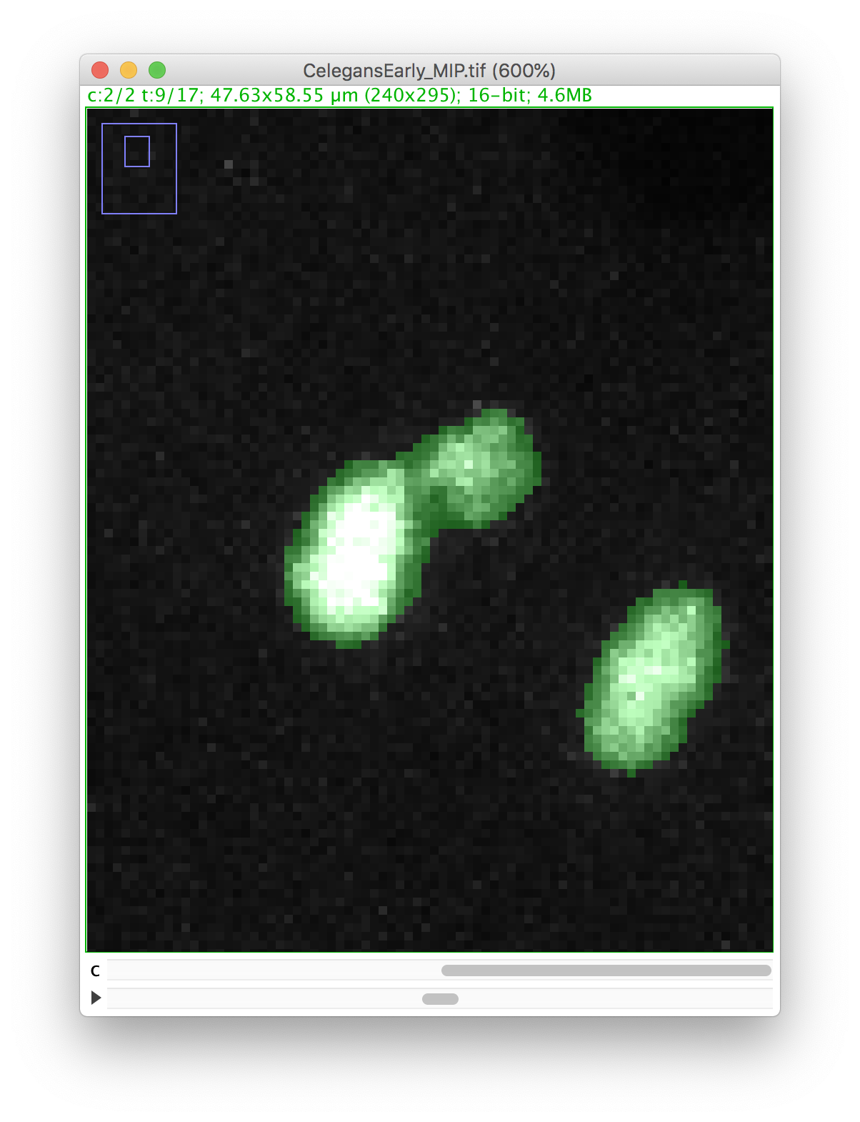
We will make a cut in the mask to separate the nucleus from the polar body. We can use the Image ROI to do so. In the ImageJ toolbar, select the line ROI tool. Double click on the color selection tool, and select the black color as the foreground color. Now draw a line that goes between the nucleus and the polar body.

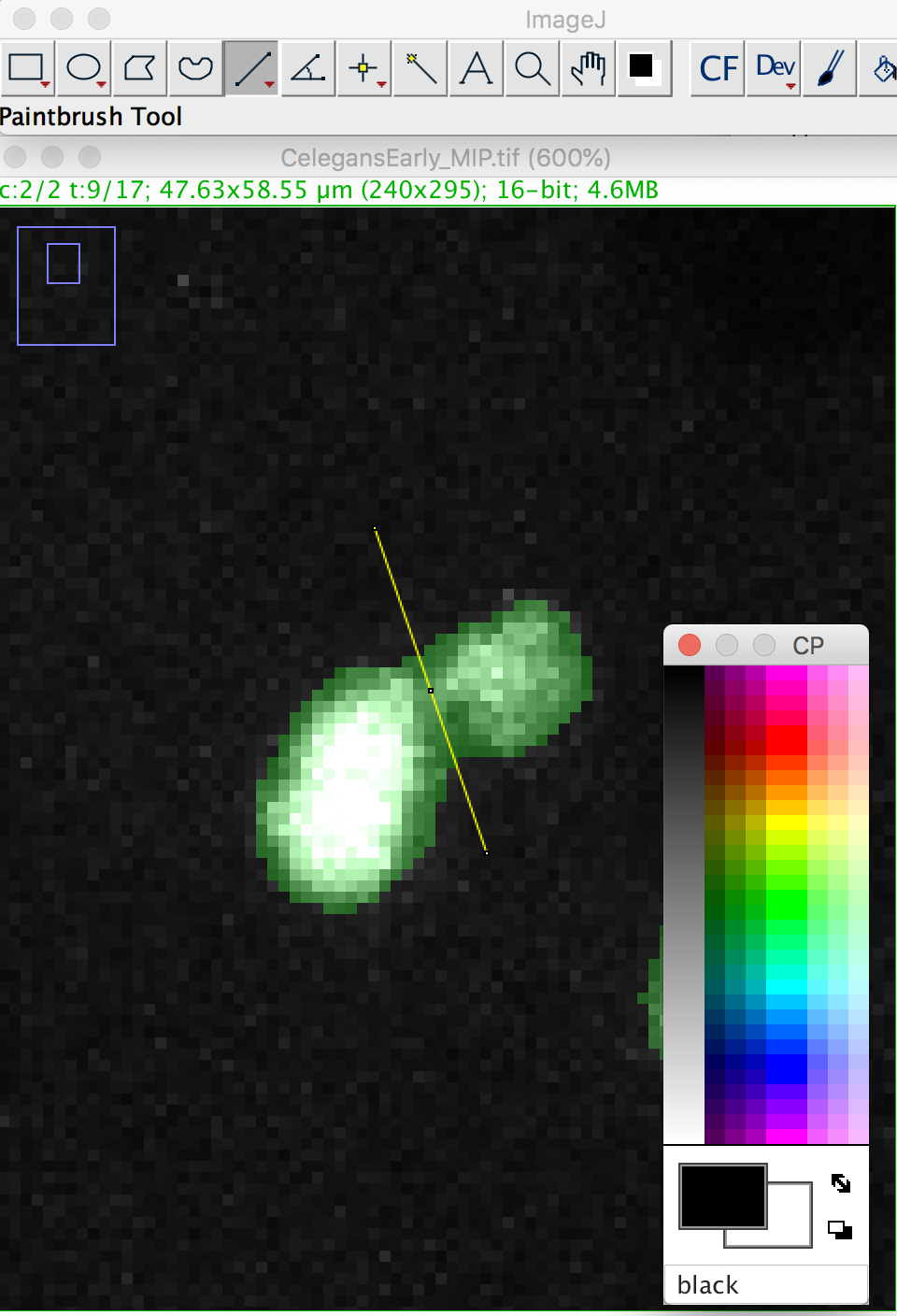
Press the D key to draw. Since we picked the black color, the pixels along the line ROI will be replaced by a pixel value of 0, cutting the mask into 2 components:

Now you can proceed with the tracking as before. The polar body and the nucleus will be segmented as two spots:

Right now, this is the only way to edit the spot contour in TrackMate. Which means it is important to get a good segmentation results before running TrackMate.

Jean-Yves Tinevez July 2021

Tutorial: Cancer cells migration

Get the tutorial dataset from Zenodo:

• Open Fiji.
• Open your image.
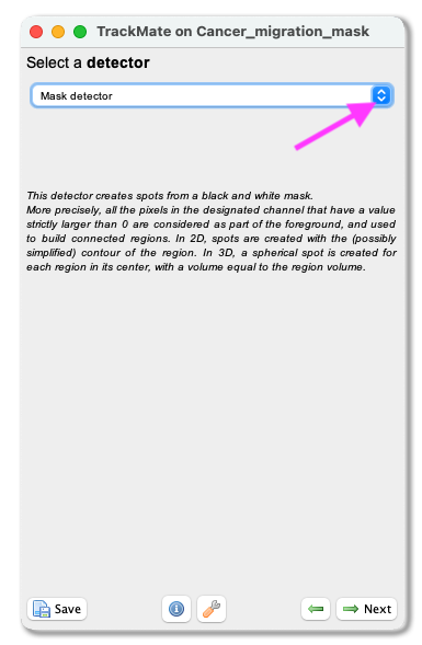
• Open TrackMate Plugins › Tracking › TrackMate. The start panel will launch, showing information about the image dimensions. Click Next.
• The “Select a detector” -panel opens. From the pull-down menu, select the Mask detector. Click Next.

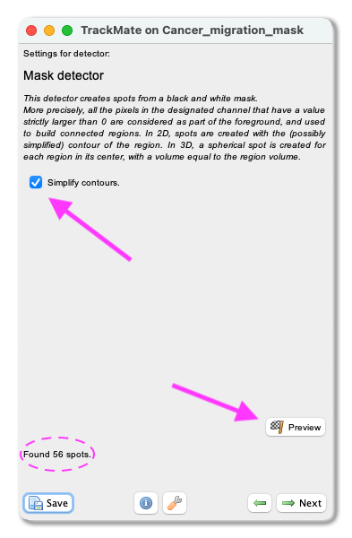
• A panel with the description of the mask detector opens. Here you can select to Simplify the contours to smooth the edges of the segmented objects. Click on Preview to see a preview of the segmentation. On the left, there will also be the number of detected objects in that field of view. Click Next. The objects are now being detected.
• When the progress bar has reached the end, click Next.
• A panel to filter the detected spots according to their quality opens (more information about this filtering can be found here. With our test image, this part can be ignored. Click Next.
• A panel to filter spots according to their properties (i.e. size, shape, location, or signal intensity) opens. With our test image, we do not need to filter any spots. Click Next.

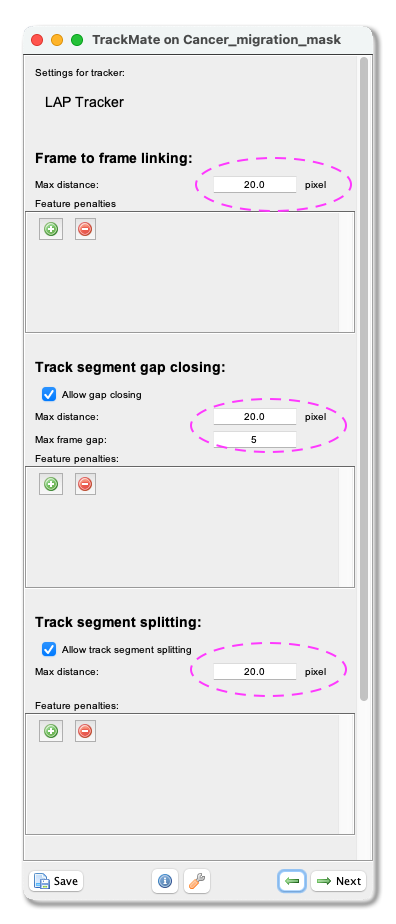
• A tracking panel opens. In this panel, you can select a method for tracking your objects. In this exercise, we use the LAP tracker. Please select it from the pull-down menu, and click Next.
• A panel to choose the LAP tracker settings opens. First, with the Frame to Frame linking parameter, you give the maximum distance to link two objects between frames. With our test image, we use 20 microns. Tick the Allow gap closing box and add values: Max distance: 20 microns and Max frame gap: 5. Next, you let TrackMate know if the tracks are allowed to split. Track splitting can occur, for example, due to cell division. Tick the box Allow track segment splitting and insert value Max distance: 20 microns. Below you will also see a setting to allow Track segment merging. This box should remain unticked as we do not expect the nuclei to merge here. Click Next.

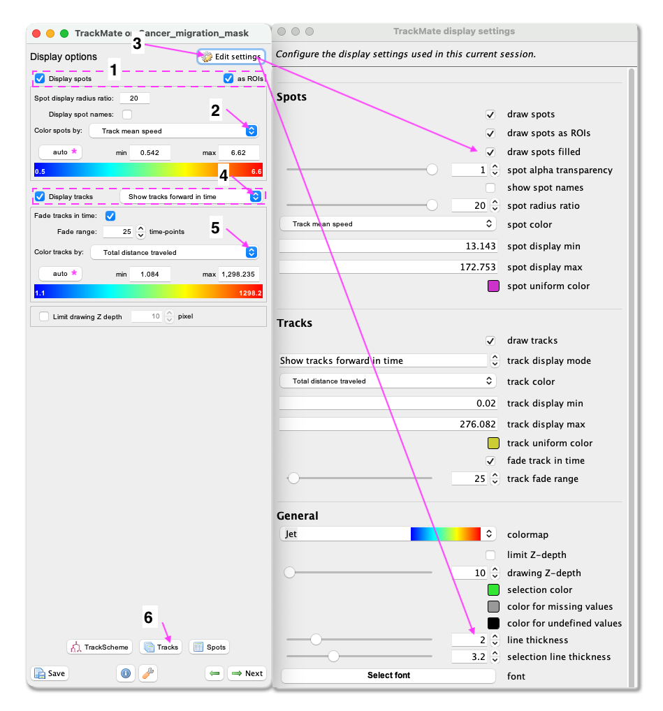
• A Track filter panel opens. In this panel, you can remove tracks according to their properties (i.e., length, speed, or location). With our test image, we do not need to filter any tracks. Click Next.

• A window with track visualization options opens. Here it is possible to edit track or object colours according to their properties. We will label the tracked objects according to their mean speed and the tracks according to the total distance travelled.
  • First, make sure that the Display spots and as ROIs boxes are ticked.
  • Select Track mean speed from the Color spots by clicking on the pull-down menu and then click auto.
  • To fill the objects with the indicative colour, click on Edit settings. This will open a new panel with display settings. Here, tick the box draw spots filled.
  • From the same panel, also set the line thickness as 2.
  • Close the Display settings window.
  • Make sure the Display tracks box is ticked.
  • From the pulldown menu, select Show tracks forward in time. This will show the future trajectories of the object movements.
  • From the Color tracks pull-down menu, select Total distance travelled. And click auto.
• In this panel, you can also export the results as .csv files. Please do so by clicking on Tracks at the bottom of the panel. A window with a lot of data will open. Ensure you export the Spots (information about the spot) and the Tracks (information about the tracks) files. Close the results window and click Next.

• In this panel, you have access to many plotting features- again, click Next.
• Here you have the possibility to do different actions. For this exercise, we will export a tracking image of our experiment. Then from the pull-down menu, select Capture overlay. After clicking on Execute, a pop-up window opens. Here you can define the time interval you want to save and click OK. TrackMate will generate a video of your experiment. Remember to save the image from File › Save as….

You can see on the resulting movie that some touching cells were incorrectly identified as one object. This is a problem with mask images. You can fix this by editing the mask as we did in the first tutorial above, or moving back to the raw image and use the StarDist detector we introduce elsewhere.

Joanna W. Pylvänäinen - July 2021