This page describes the segmentation function of the CIP scripting package
One can found additional information on the function parameters (type, optional/required, positional/named) on the parameters documentation page.
To access another category of CIP functions: Format, Filter, Math, Segment, Assess, Experimental.
threshold
Description
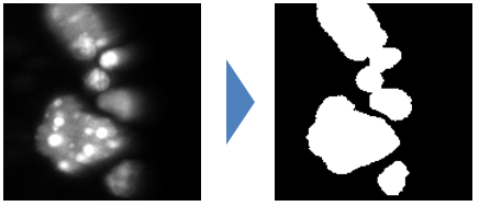
this function creates a binary image from an input graylevel image
Signatures
outputImage = cip.threshold( inputImage* , threshold*)
outputImage, threshold = cip.threshold( inputImage* , method*, output)
Input
inputImage* : the image to process
threshold* : a scalar value use to threshold the image
method* : a string in {‘huang’, ‘ij1’, ‘intermodes’, ‘isoData’, ‘li’, ‘maxEntropy’, ‘maxLikelihood’, ‘mean’, ‘minError’, ‘minimum’, ‘moments’, ‘otsu’, ‘percentile’, ‘renyiEntropy’,’rosin’, ‘shanbhag’, ‘triangle’, ‘yen’}.
output : a string in {‘image’, ‘value’, ‘both’}defining the type of output.
Output
outputImage: the processed image. threshold: the threshold value calculated for the image and method provided as input.
Example
img2 = cip.threshold( img1 , 500 )

Implementation
the threshold method wraps ops threshold methods
label
Description
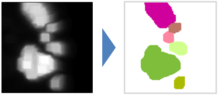
This function threshold an image and label its connected component (i.e. it sets the pixels of each region to a distinct integer value).
Signature
outputImage = cip.label( inputImage* , threshold)
Input
inputImage* : the image to process
threshold : a scalar value to threshold the image. If the input image is binary no threshold is needed
Output
outputImage: a label map (an image with background 0 and where each identified region has a distinct integer value).
Example
img2 = cip.label( img1 )

Implementation
The labeling is performed our custom implementation. It uses a union find approach relying pixel runs to speed up to labeling process. The source code is available on github. The principle of the algorithm was described in [1].
[1] Cabaret, Laurent, Lionel Lacassagne, and Louiza Oudni. “A review of world’s fastest connected component labeling algorithms: Speed and energy estimation.” Design and Architectures for Signal and Image Processing (DASIP), 2014 Conference on. IEEE, 2014.
maxima
Description
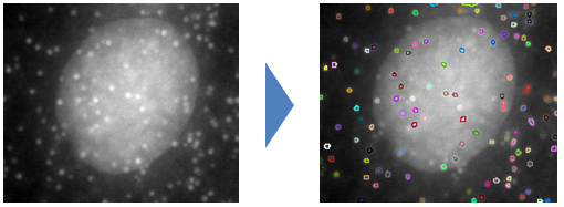
This function detects the intensity maxima of an imaget and return a labeled image of these maximage.
Signature
outputImage = cip.maxima( inputImage* , threshold, heightMin, areaMin, distanceMin, scaleMin, scaleMax, method, pixelSize)
Input
inputImage* : the image to process
threshold : the minimum intensity of the maxima
heightMin : the minimum dynamics of the maxima peak. defining this value triggers an extended maxima detection unless scale parameters are defined
areaMin : the minimum area in pixel of the maxima peak. if heightMin is defined this value is ignored.
areaMin : the minimum distance in pixel between the maxima. if heightMin or areaMin are defined this value is ignored.
scaleMin : if that value is defined a multiscale maxima detection is ran and this value represent the minimum scale of the maxima
scaleMax : if that value is defined a multiscale maxima detection is ran and this value represent the maximum scale of the maxima
method : a string in {‘classic’, ‘height’, ‘area’, ‘distance’, ‘multiscale’} defining the method to be used for maxima detection
pixelSize : a scalar or a list of scalar defining pixel size to use for multiscale detection. by default this value is 1
Output
outputImage : a label image of the detected maxima
Experimental feature
For the multiscale maxima method it is possible to use a parameter defining the type of output returned by the function
output : a string in {‘image’, ‘measure’, ‘both’}, the default value is ‘image’. If the parameter value is ‘image’ the function return a labelMap image. If the value is ‘measure’ the function a measure table indicating object position and scale. The idea is to give more flexibility in the visualisation of the detections. Eventually returning sphere regions with appropriate radii could be more convenient as they could be visualized right away with cip.show
Example
img2 = cip.maxima( img1 , 'hmin', 200 )

the illustration above show the contour of the detected region on top of the original data
Implementation
Each maxima detection method rely on a custom implementation
Classic method is a union find implementation of maxima detection
Height and Area methods are derived from attribute filtering approaches [1] simply using a different attribute peak height or area as criteria to merge peaks and stop their extension.
Distance is simpler but efficient approach that pass a filter window over the image and check is all pixel values in the window are lower or equal to the center pixel. This method can make errors if image contains plato.
MultiScale method builds a difference of gaussian pyramid and detection in that scale space. The implementation principle is well described in [2].
[1] Meijster, A., & Wilkinson, M. H. (2002). A comparison of algorithms for connected set openings and closings. IEEE Transactions on Pattern Analysis and Machine Intelligence, 24(4), 484-494.
[2] Lowe, D. G. (2004). Distinctive image features from scale-invariant keypoints. International journal of computer vision, 60(2), 91-110.
watershed
Description
Watershed algorithm partitions an image in regions and outputs a label image of these regions. Initialized with image maxima or or user defined regions the algorithm grow these seed regions following the shape of, i.e. flooding, intensity peaks.
Signature, Input 1
outputImage = cip.watershed( inputImage* , threshold, heightMin, peakFlooding, method)
inputImage* : the image to process
threshold : an intensity value at which the region growing will stop
heightMin : the minimum dynamics of the maxima used to initialize the watershed. default is 5 percent of the image dynamics
peakFlooding : a percentage of peak flooding. 0 mean the region will be reduced to its maxima while 100 give the full region.
method : a string in {‘gray’,’binary’} defining if the watershed is calculated on the gray level image or a distance map
Signature, Input 2
outputImage = cip.watershed( inputImage* , seed, threshold)
inputImage* : the image to process
seed : a label image of the region that will initialize the watershed process
threshold : an intensity value at which the region growing will stop
Output
outputImage : a label image of the detected maxima
Example
img2 = cip.watershed( img1 , 'threshold', 500, 'hmin', 300 )
In that example the starting point of the watershed are the extended maxima of the input image.

Implementation
Both seeded watershed and H-watershed are implemented based on the image foresting transform approach [1]. The H-watershed adds the construction of a hierarchical tree of segment that can be used in further applications. Both implementations can be found here and there
[1] Lotufo, R. D. A., Falcão, A. X., & Zampirolli, F. A. (2002). IFT-watershed from gray-scale marker. In Computer Graphics and Image Processing, 2002. Proceedings. XV Brazilian Symposium on (pp. 146-152). IEEE.