The content of this page has not been vetted since shifting away from MediaWiki. If you’d like to help, check out the how to help guide!
Introduction
In this tutorial we describe step by step how to compare the performance of different classifiers in the same segmentation problem using the Trainable Weka Segmentation plugin.
Most of the information contained here has been extracted from the WEKA manual for version 3.7.3, chapter 6.
Starting the plugin
To get started, open the 2D image or stack you want to work on and launch the Trainable Weka Segmentation plugin (under Plugins › Segmentation › Trainable Weka Segmentation):
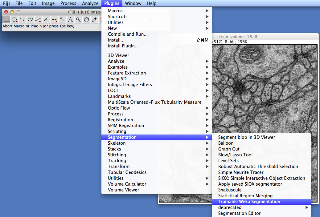
For this tutorial, we used one of the TEM sections from Albert Cardona’s public data set.
After loading, the main GUI of the plugin will pop up: 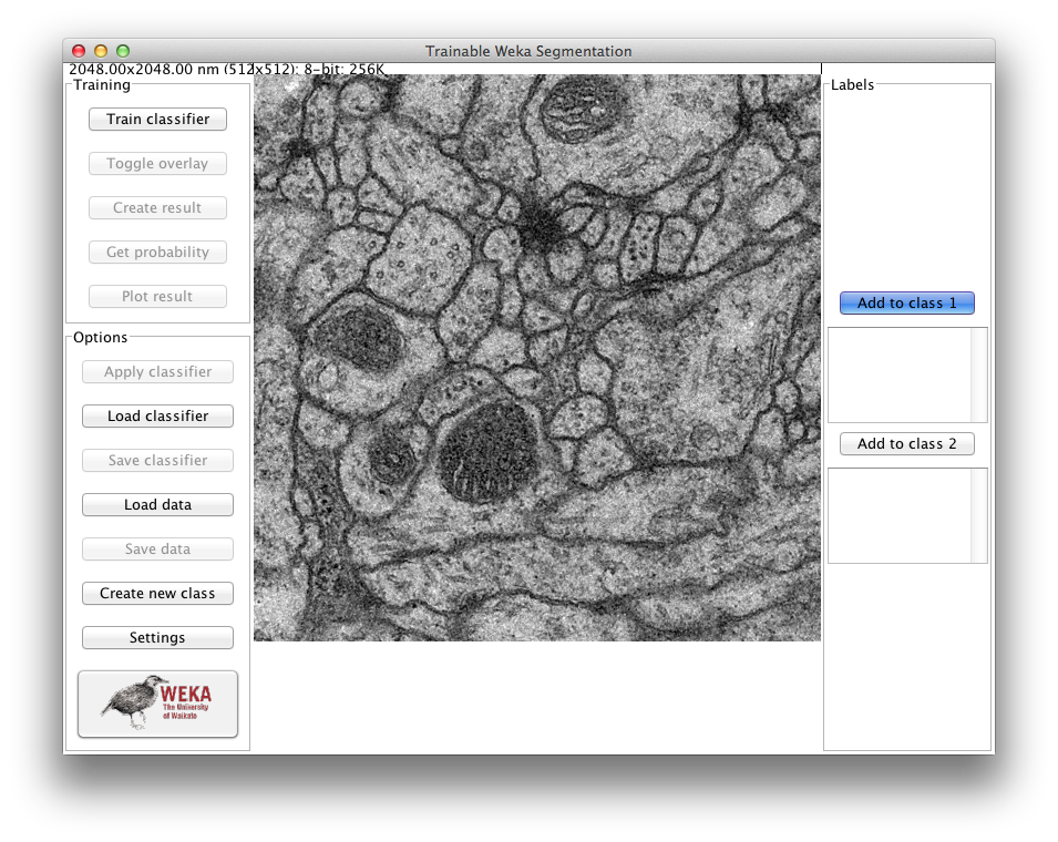
Gathering training samples
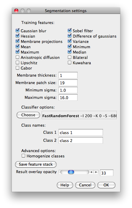
First of all, we select the features (filters) that we want to use to perform the segmentation. For that, we will click on “Settings”, select the corresponding features on the Settings dialog, and click “OK”:
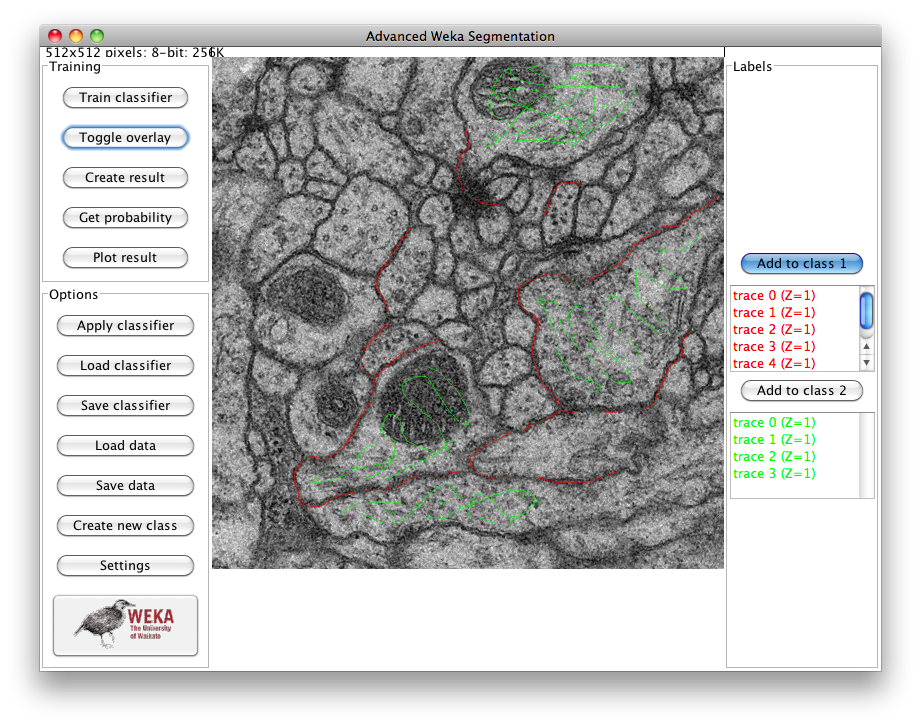
After that, we use the selection tools to trace samples of both classes. By default, the “freehand” line is selected, but you can use any of the available selection tools to mark areas on the image and then add them to any of the classes by click on the “Add to class [1/2]” buttons. In our example, we use the two classes to differentiate between membrane areas (in red, class 1) and the rest of the image (in green, class 2):
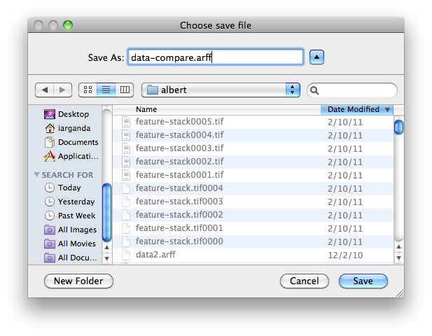
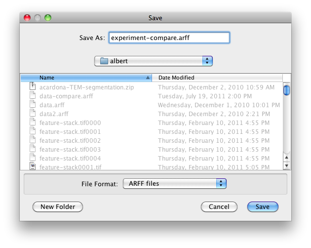
Once we are satisfied with the amount of samples, we save the data into an ARFF file, the format WEKA understand. For that, we click on “Save data” and select the output path and file name (“data-compare.arff” in our case):
Working with the WEKA Experimenter
In order to use the data we just saved for comparing classifiers, we need to open the WEKA Experimenter. For that, we first click on the WEKA button of the plugin GUI (last button of the left panel). Then the Weka GUI Chooser will pop up:
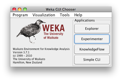
We click on “Experimenter” and the Weka Experiment Environment GUI will pop up:
New experiment
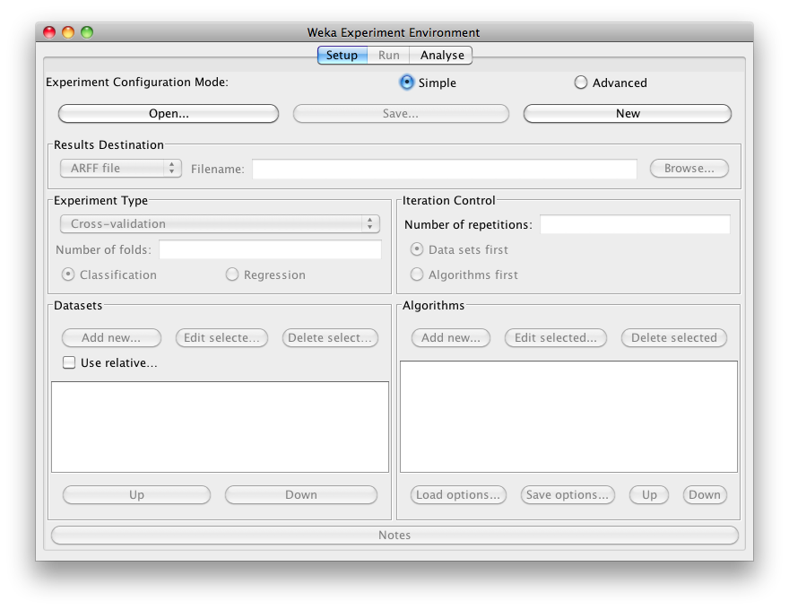
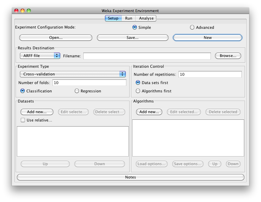
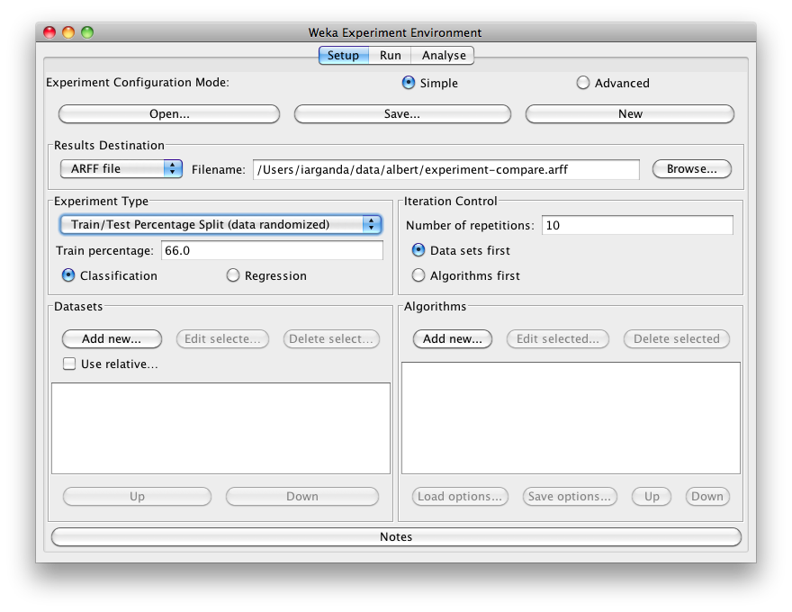
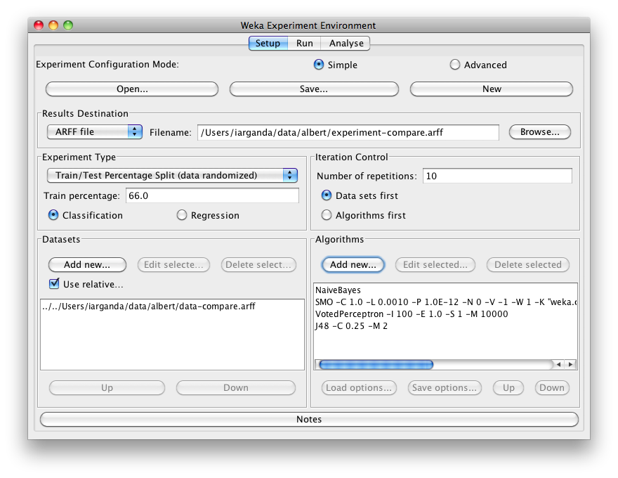
In this tutorial we use the “Simple” configuration mode. After clicking New, default parameters for an Experiment are defined:
Results destination
By default, an ARFF file is the destination for the results output. But you can choose between
- ARFF file
- CSV file
- JDBC database
CSV is similar to ARFF, but it can be used to be loaded in an external spreadsheet application. If the file name is left empty a temporary file will be created in the TEMP directory of the system. If one wants to specify an explicit results file, click on Browse and choose a filename. In our case, we set the filename to experiment-compare.arff:
Click on Save and the name will appear in the edit field next to ARFF file.
Experiment type
The user can choose between the following three different types
- Cross-validation (default) performs stratified cross-validation with the given number of folds.
- Train/Test Percentage Split (data randomized) splits a dataset according to the given percentage into a train and a test file (one cannot specify explicit training and test files in the Experimenter), after the order of the data has been randomized and stratified:
- Train/Test Percentage Split (order preserved) because it is impossible to specify an explicit train/test files pair, one can abuse this type to un-merge previously merged train and test file into the two original files (one only needs to find out the correct percentage).
Additionally, one can choose between Classification and Regression, depending on the datasets and classifiers one uses. Classification is selected by default.
Note: if the percentage splits are used, one has to make sure that the corrected paired T-Tester still produces sensible results with the given ratio.
Datasets
One can add dataset files either with an absolute path or with a relative one. The latter makes it often easier to run experiments on different machines, hence one should check Use relative paths, before clicking on Add new…:
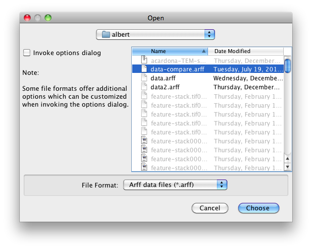
In this example, we open the albert directory and choose the data-compare.arff dataset.
After clicking Open the file will be displayed in the datasets list. If one selects a directory and hits Open, then all ARFF files will be added recursively. Files can be deleted from the list by selecting them and then clicking on Delete selected.
Algorithms
New algorithms can be added via the Add new… button. Opening this dialog for the first time, ’ ZeroR’ is presented, otherwise the one that was selected last:
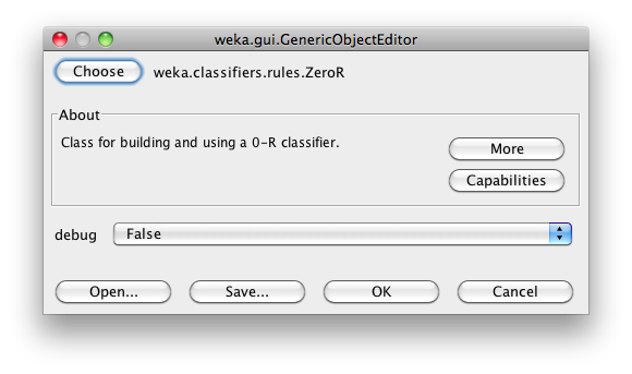
With the Choose button one can open the GenericObjectEditor and choose another classifier:
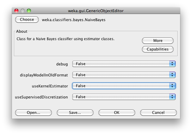
The Filter… button enables one to highlight classifiers that can handle certain attribute and class types. With the Remove filter button all the selected capabilities will get cleared and the highlighting removed again.
Additional algorithms can be added again with the Add new… button. After setting the classifier parameters, one clicks on OK to add it to the list of algorithms. In our example, we add NaiveBayes, SMO, VotedPerceptron and J48:
With the Load options… and Save options… buttons one can load and save the setup of a selected classifier from and to XML. This is especially useful for highly configured classifiers (e.g., nested meta-classifiers), where the manual setup takes quite some time, and which are used often.
One can also paste classifier settings here by right-clicking (or ⌥ Alt + ⇧ Shift +  Left Click) and selecting the appropriate menu point from the popup menu, to either add a new classifier or replace the selected one with a new setup. This is rather useful for transferring a classifier setup from the Weka Explorer over to the Experimenter without having to setup the classifier from scratch.
Saving the setup
For future re-use, one can save the current setup of the experiment to a file by clicking on Save… at the top of the window:
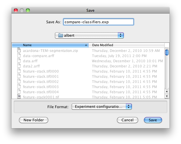
By default, the format of the experiment files is the binary format that Java serialization offers. The drawback of this format is the possible incompatibility between different versions of Weka. A more robust alternative to the binary format is the XML format.
Previously saved experiments can be loaded again via the Open… button.
Running an experiment
To run the current experiment, click the Run tab at the top of the Experiment Environment window. The current experiment performs 10 runs of Train/Test percentage split (with data randomized) on the TEM image dataset using the NaiveBayes, SMO, VotedPerceptron and J48 schemes:
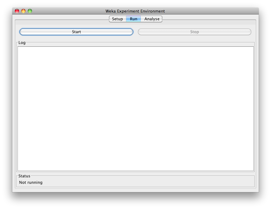
Click Start to run the experiment:
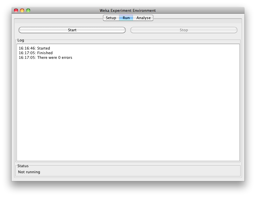
If the experiment was defined correctly, the 3 messages shown above will be displayed in the Log panel. The results of the experiment are saved to the dataset experiment-compare.arff.
Analysing results
Setup
To analyse the results, select the Analyse tab at the top of the Experiment Environment window.
Click on Experiment to analyse the results of the current experiment:
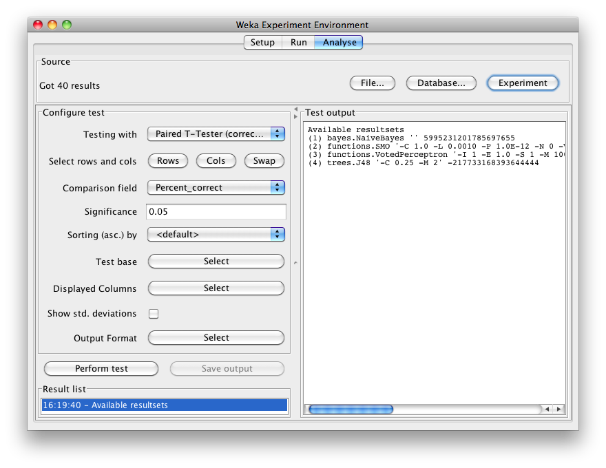
The number of result lines available (Got 40 results) is shown in the Source panel. This experiment consisted of 10 runs, for 4 schemes, for 1 dataset, for a total of 40 result lines. Results can also be loaded from an earlier experiment file by clicking File and loading the appropriate .arff results file.
Select the Percent correct attribute from the Comparison field and click Perform test to generate a comparison of the 4 schemes:
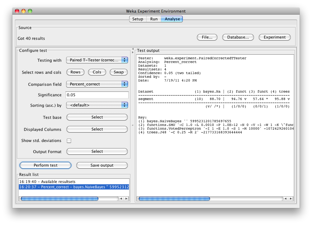
The schemes used in the experiment are shown in the columns and the datasets used are shown in the rows.
The percentage correct for each of the 4 schemes is shown in each dataset row: 88.70% for NaiveBayes, 94.76% for SMO, 57.64% for VotedPerceptron and 95.88% for J48. The annotation v or * indicates that a specific result is statistically better (v) or worse (*) than the baseline scheme (in this case, NaiveBayes) at the significance level specified (currently 0.05). The results of both SMO and J48 are statistically better than the baseline established by NaiveBayes. At the bottom of each column after the first column is a count (xx/ yy/ zz) of the number of times that the scheme was better than (xx), the same as (yy), or worse than (zz), the baseline scheme on the datasets used in the experiment. In this example, there was only one dataset and SMO was better than NaiveBayes once and never equivalent to or worse than NaiveBayes (1/0/0); J48 was also better than NaiveBayes on the dataset, and VotedPerceptron was worse.
The standard deviation of the attribute being evaluated can be generated by selecting the Show std. deviations check box and hitting Perform test again. The value (10) at the beginning of the segment row represents the number of estimates that are used to calculate the standard deviation (the number of runs in this case).
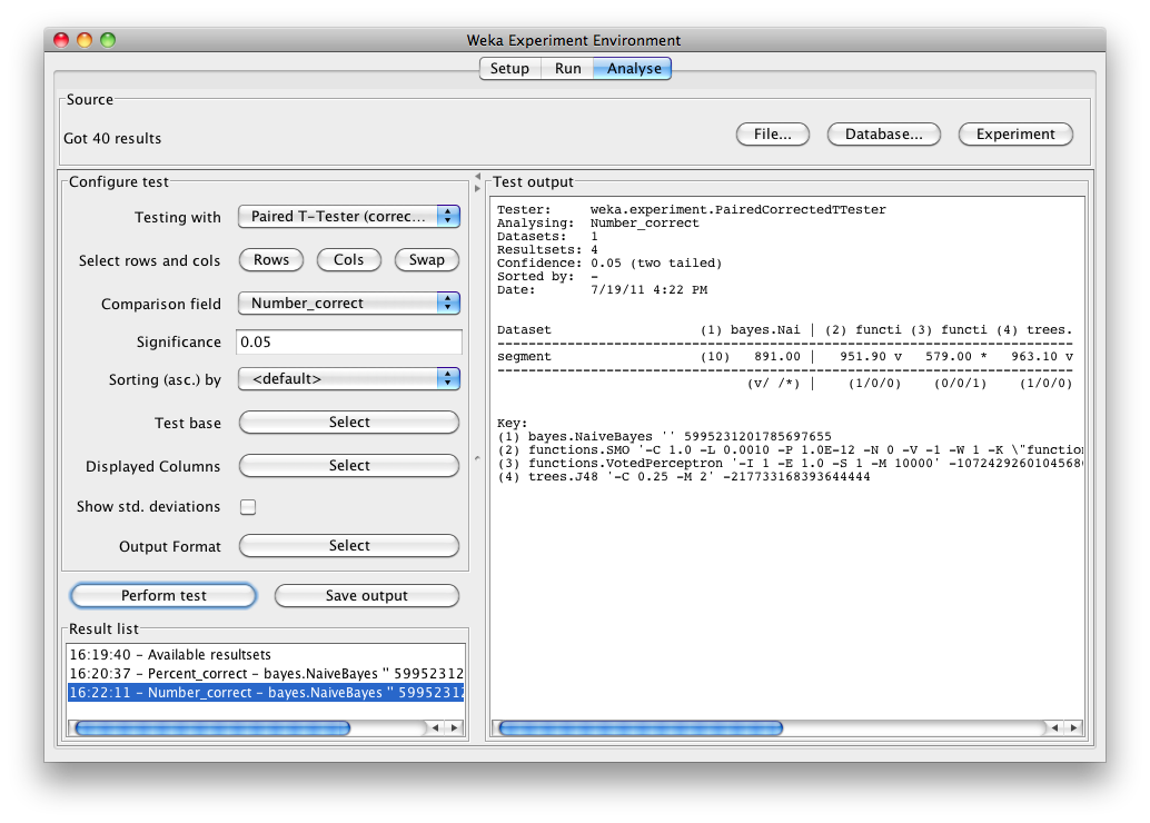
Selecting Number correct as the comparison field and clicking Perform test generates the average number correct (out of 975 test patterns - 33% of 2954 patterns in the segment dataset).
Clicking on the button for the Output format leads to a dialog that lets you choose the precision for the mean and the std. deviations, as well as the format of the output. Checking the Show Average checkbox adds an additional line to the output listing the average of each column. With the Remove filter classnames checkbox one can remove the filter name and options from processed datasets (filter names in Weka can be quite lengthy). The following formats are supported:
- CSV
- GNUPlot
- HTML
- LaTeX
- Plain text (default)
- Significance only
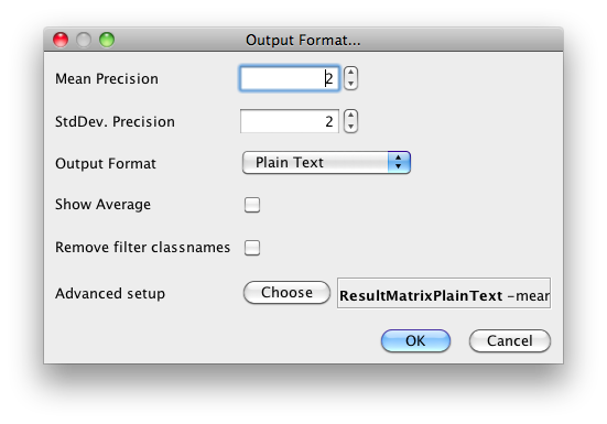
To give one more control, the “Advanced setup” allows one to bring up all the options that a result matrix offers. This includes the options described above, plus options like the width of the row names, or whether to enumerate the columns and rows.
Saving the Results
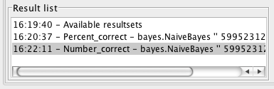
The information displayed in the Test output panel is controlled by the currently selected entry in the Result list panel. Clicking on an entry causes the results corresponding to that entry to be displayed.
The results shown in the Test output panel can be saved to a file by clicking Save output. Only one set of results can be saved at a time but Weka permits the user to save all results to the same file by saving them one at a time and using the Append option instead of the Overwrite option for the second and subsequent saves.