The problem with tracking algorithms is that they always give an answer.
This answer can be completely irrelevant, even non-physical, and there is no built-in flags that would indicate something wrong. The best way to avoid basing your downstream analysis on faulty tracking results is to know in what situation the tracker works the best, and what are its limitations. This is the aim of this page for the trackers and detectors shipped with TrackMate.
The ISBI 2012 single particle challenge
In 2011-2012, an ISBI Grand Challenge was organized for the Single-Particle Tracking algorithms. Though TrackMate does not offer a completely new algorithm, product of an original Research work, we took the chance and participated in the challenge. The results and the methodology to compute the accuracy of a tracking algorithms were published1 thereafter.
Unsurprisingly, we did not score amongst the best. At the time, TrackMate was in version 1.1, and ship a stripped down version of the better performing Jaqaman et al. LAP framework2. See the LAP trackers section for algorithm details. Plus, TrackMate was was young at the time, and some bugs did not help.
TrackMate v2.7.x series accuracy against the ISBI dataset
From v2.7.x, TrackMate ships a new tracker that can deal specifically with linear motion. We thought it was the right time to re-run the accuracy assessment with the ISBI challenge data. The people behind Icy offered the website to host the challenge data, and it is still available today for download.
The figures below shows the comparison of accuracy for the 3 classes of tracking algorithms available in TrackMate:
- The LAP framework derived from Jaqaman et al.2.
- The linear motion tracker based on Kalman filter.
- The plain Nearest neighbor tracker for reference.
Scenarios
It’s best to directly read the paper1 to know what is behind these measures, but here is a brief survey of how they are done. The ISBI dataset covers four scenarios:
|
Scenario name |
Particle shape |
Motion type |
|---|---|---|
|
Slightly elongated shape to mimic MT tip staining. |
Roughly constant velocity motion. |
|
|
Spherical. |
Tethered motion: switch between Brownian and directed motion with random orientation for the later. |
|
|
Switch between Brownian and directed motion with fixed orientation for the later. |
For each scenario, images covers several particle density:
- low: 60-100 / frame
- mid: 400-500 / frame
- high: 700-1000 / frame
to check how a tracking algorithm behaves when particles get very dense.
Also, particles SNR spans several values: 1, 2, 4, 7 (plus 3 for the RECEPTOR scenario). As said on the challenge page: “SNR=4 is a critical level at which methods may start to break down”.
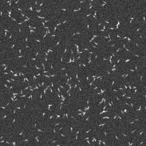
Example images from the challenge dataset
Below are shown typical images taken from the challenge.
Varying particle density
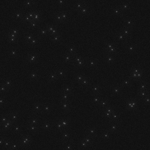
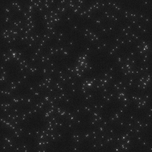
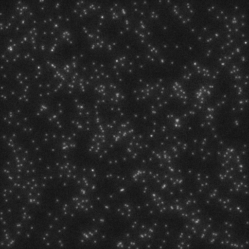
Contrast stretched to the 0-150 8-bit range.
Varying particle SNR
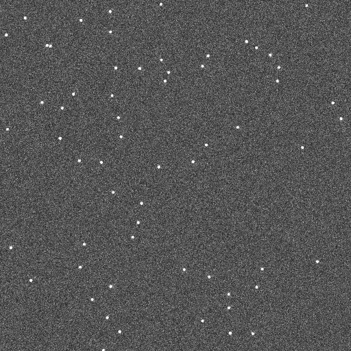
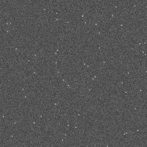
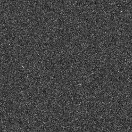
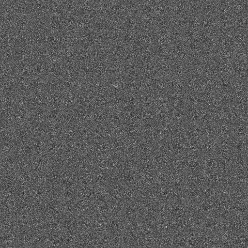
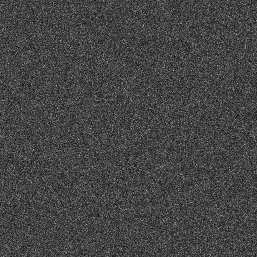
Contrast stretched to the 0-50 8-bit range.
The MICROTUBULE scenario particle shape
Accuracy measurements
For each scenario and condition, the method returns numerous values that characterizes the accuracy of a tracking algorithm. They are detailed on this technical paper. We plot below only three of them:
- The Jaccard similarity between tracks, that quantifies how well the tracks returned by the algorithm match the ground truth. This value assesses the accuracy of the spot tracker you pick in TrackMate. It ranges from 0 (terrible) to 1 (found tracks = ground truth).
- The Jaccard similarity between detections, that quantifies how well the particle detected by the detection algorithm match the ground truth. It depends strongly on the spot detector you pick in TrackMate, and ranges from 0 to 1 like the above quantity.
- The RMSE of detection positions that quantifies how precise is the location of the detected particles. The smaller the better.
I fully relied on Icy to compute these values. TrackMate ships an action that exports tracking results to the XML format imposed by the ISBI challenge, and that can be found here. I generated these files for all the conditions of a scenario, and used the Icy ISBI challenge scoring plugin to yield metrics. I then used MATLAB to plot them.
Parameter used
Unless otherwise specified below, I always used the LoG detector as a spot detector, with an estimated particle diameter of 2, and used sub-pixel accuracy. For SNR below 4, this detector was completely confused and the detection results are dominated by noise. I did not make anything special to improve its sensitivity below this limit.
When the histogram of detection quality returned by the detector as not bimodal, I pick a quality threshold that yielded approximately the expected number of particles in the sequence.
The three spot trackers were configured as indicated in the table below. It’s not very sensible to keep always the same parameter across different scenario, but with what you can tune in TrackMate, there is little room for fine-tuning.
| Spot tracker | Parameter | Value |
|---|---|---|
| Kalman tracker (linear motion) | Initial search radius | 10 |
| Search radius | 7 | |
| Max frame gap | 3 | |
| LAP tracker (Brownian motion) | Max linking distance | 7 |
| Max gap-closing distance | 10 | |
| Max frame gap | 3 | |
| Nearest neighbor | Max search distance | 10 |
Finally, for SNR<4, I filtered out tracks that had less than 4 detections.
Results
The results for each scenario is presented and commented below. Since we used the same detector for all scenarios, all the measures have s common shape for their dependence on SNR.
Basically, accuracy is the same for SNR ≥ 3. Below SNR = 2 included, the detector is unable to reliably finds all the particles. For a SNR of 2, it still finds a subset of correct particles, amongst the brightest. At a SNR of 1, detection results are dominated by spurious detections, and the particle linking algorithm performance does not matter anymore. All are equally bad, since they track the wrong particles.
Microtubule scenario
This scenario probes how well the TrackMate algorithms fare against a roughly constant velocity motion model. Unsurprisingly, the linear motion tracker performs the best and resits well against high density of particles.
The LAP tracker does not perform well, even in the ideal case, as it expects the average particle position to be constant at least on short timescales, when it does not. Therefore, it performance approaches the worst-case scenario given by the nearest-neighbor search algorithm.
The RMSE on particle position is the worst here over the 4 scenarios. This is the obvious consequence of the particle shape, which is asymmetric and elongated, when the LoG detector expects bright blobs. Still, this does not affect tracking results.
Receptor scenario
TrackMate does not have a particle linking algorithm that specifically address this scenario. The motion model switches from Brownian motion to linear motion, and we have algorithm that deal with one or the other. It is no surprise therefore to find that they all perform similarly.
Fortunately, accuracy values are rather good and do not break down too much against particle number. We also see that the linear motion tracker behaves slightly better than the rest in all conditions.
Vesicle scenario
The motion model of this scenario is the pure Brownian motion. Unsurprisingly the LAP tracker behaves the best as it models precisely this situation. The linear motion tracker is confused by the constant direction changed generated by the random motion, and is superseded even by the nearst neighbor search.
Virus scenario
As for the receptor scenario, TrackMate does not have a specific tracker for this scenario. The main difference with the receptor scenario is that the linear motion part of the trajectories are all following the same direction. Again, TrackMate cannot exploit this bit of information, but it is enough to change what is the better performing algorithm (compared to the receptor scenario).
Also, this scenario was the only one to ship 3D data over time. Thanks to ImgLib2 dimensional genericity, TrackMate does not mind.
Comments
These results should help you pick the right algorithm for your problems, and maybe encourage you to implement your own. As said before, a deeper interpretation of these metrics in the general case is found in the original paper1. Here are a few things specific to the current version of TrackMate.
The parameters and strategy used for this accuracy assessment are pretty basic and unelaborated. This way, results give the ‘raw’ accuracy, before a user exploits the deeper specificity of their problem. The two sections below quickly list what we could have done and could not have done even if we wanted to improve results.
What was in the challenge that TrackMate did not exploit?
We saw that at low SNR, the detection step dominates and its inability to robustly detect faint particles is the cause for low scores. Here I did not try to improve the detection results via pre-processing. One could have denoised the image, or averaged succeeding frames to improve the SNR. Or a better detector could have dealt with low SNR in a better way (the Low Light Tracking Tool maybe).
What is in TrackMate that we could not exploit for the challenge?
The LAP trackers were the first trackers to be shipped with TrackMate. They are a stripped down version of. They are based solely on square distance costs (Brownian motion), but they can be modulated by a penalty factor based on numerical features. For instance, the cost to link two particles can be penalized if their mean intensity is too different.
The challenge data does offer that possibility: all particles have roughly the same shape and intensity (modulo some minor variations in SNR). An exception is the MICROTUBULE scenario, where particles have an elongated shape. Therefore, we could have computed an orientation for them, and penalize two particles with different orientation (assuming - correctly - that orientation remains roughly the same between two frames).