The content of this page has not been vetted since shifting away from MediaWiki. If you’d like to help, check out the how to help guide!
Overview
MiNA is a simplified workflow for analyzing mitochondrial morphology using fluorescence images or 3D stacks in Fiji. The workflow makes use of ImageJ Ops, 3D Viewer, Skeletonize (2D/3D), Analyze Skeleton1, and Ridge Detection23. In short, the tool estimates mitochondrial footprint (or volume) from a binarized copy of the image as well as the lengths of mitochondrial structures using a topological skeleton. The values are reported in a table and overlays (or a 3D rendering) are generated to assess the accuracy of the analysis.
Installation
To install MiNA and the additional plugins, scripts, and macro tools our lab uses bundled with it, we suggest adding our update site (“StuartLab”). By this method, you will receive automatic updates everytime the updater is run ensuring you get new features and bug fixes as soon as they are available. To add the update site in your installation of Fiji:
- Open Fiji.
- Run the updater (Help → Update…).
- Navigate to the update site manager (Manage update sites).
- Add the “StuartLab” and “Biomedgroup” sites by checking the checkbox beside the site.
- Close the site manager dialog (Close).
- Apply the changes (Apply changes).
Processing Pipeline and Usage
Determing the Area/Volume of Mitochondria

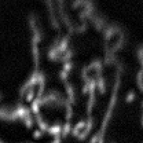
MiNA extracts morphological information from two simplifications of the image. For demonstration purposes, we will be using the micrograph crop in Figure 1. One is a binary representation, which simply represents pixels as containing signal or being background. This is generated by automatic thresholding, a good overview of which available on the Auto Threshold page. There are many thresholding methods available through ImageJ Ops. So far, only global thresholds are provided, though local thresholds will be incorporated eventually. The methods included are listed below. If you find an issue arises using a specific thresholding method, please open an issue using the GitHub issue tracker (only a subset were tested).
- huang 4
- ij15
- intermodes6
- isoData7
- li8
- maxEntropy9
- maxLikelihood
- mean10
- minError11
- minimum12
- moments13
- otsu (default)14
- percentile15
- renyiEntropy16
- rosin
- shanbhag17
- triangle18
- yen19

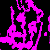
Once the image has been binarized, the area or volume can be estimated by simply counting the number of signal positive pixels/voxels and multiplying by the area or volume of the pixel/voxel approximated as a rectangle or rectangular prism. Figure 2 illustrates an image after thresholding. In the binarized image, magenta represents the signal positive pixels, while the background pixels are black. This binarized copy is overlaid upon the original image after processing as an accuracy/artifact check measure. The area or volume of the image occupied by signal is returned as the mitochondrial footprint, the units of which will depend on how the image has been calibrated. You can check the image calibration under Image → Properties.
Estimating Mitochondrial Lengths and Branching
A second simplification is made to the image for the purpose of estimating the lengths of mitochondrial structures and the degree of branching. The simplification is the generation of a morphological skeleton from which polylines can be extracted and analyzed (as is accomplished by the Analyze Skeleton20 plugin). The skeleton itself can be generated in two ways. The first, iterative thinning, is the method used in the original macros and produces a skeleton by iteratively removing outer pixels until a one pixel wide structure remains. This is accomplished through the Skeletonize (2D/3D) plugin’s methods and has the added benefit of operating on 3D datasets as well as 2D. To use this method, mitochondria must be well resolved such that the individual mitochondria can be completely segmented from each other when the binary is generated.
Ridge detection has also been incorporated and generates a skeleton not from a binary but by using the fluorescence intensity itself. This is accomplished through the methods afforded by the Ridge Detection2122 plugin. Ridge detection requires additional parameters, which are to be supplied at the prompt. It is advantageous to tune the parameters in the Ridge Detection plugin itself as it provides a preview mode. The parameters used are high contrast, low contrast, line width, and minimum length. Note that for Ridge Detection preview, images must be 8-bit. If your image is not 8-bit you must convert it using Image → Type. If using MiNA, there is no need to convert; it will be done automatically.

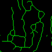
The information extracted from the morphological skeleton is the mean, median and standard deviation of the branch lengths for each independent feature and the number of branches in each network. No data is removed, so a feature that is simply a vertex, a rod without any branching points, or a complicated highly branched network will all be used when determining the length and branch count parameters. The information is summarized from the output of the Analyze Skeleton23 plugin methods. Once processed, the skeleton, an example of which is shown in Figure 3, is overlaid in green for assessing the faithfulness of the skeleton.
It is mandatory that users ensure the morphological skeleton can be accurately generated for their system of interest. The analysis tool is typically not suitable for extremely clumped mitochondria, poorly resolved images, or images with low contrast. The overlay (or 3D render) is intended as a means to assess whether the model from which the parameters are generated will be meaningful or not.
Input Parameters

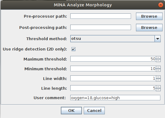
A user interface prompts the user to supply a number of parameters summarized below. The interface is displayed in Figure 4.
| Parameter: | Description: |
|---|---|
| Pre-processor path (optional) | The path to an ImageJ script or macro to run before the analysis is run. This is typically used to run user defined preprocessing operations on the image before it is analyzed, such as expanding the histogram range, reducing noise by filtering, or deconvolving the image. It is optional. |
| Post-processor path (optional) | The path to an ImageJ compatible script or macro to be run when the analysis completes. This can be used to trigger saving a copy of the data, plotting the current data stored in the ResultsTable window, and much more. It is optional. |
| Threshold method | The algorithm used to determine the threshold value. Note that the analysis expects a positive signal. The analysis will fail if the intensity is inverted. |
| Use ridge detection (2D only) | Check if ridge detection is to be used. If it is unchecked, the analysis will proceed with iterative thinning to generate the morphological skeleton. Note that ridge detection is only available for 2D images currently. |
| High contrast | Only required when using ridge detection! This defines the High Contrast value for the ridge detection plugin. |
| Low contrast | Only required when using ridge detection! This defines the Low Contrast value for the ridge detection plugin. |
| Line width | Only required when using ridge detection! The expected width of the line like mitochondrial features. |
| Line length | Only required when using ridge detection! The minimum line length to be included in the analysis. Setting this above 0 can aid in removing spurious small lines. |
| User comment | A user comment to store in the table. This supports key-value pairs, which is useful for storing condition information. For example, if I wanted a column “oxygen” and a column “glucose” to store the culture conditions, I could use the comment “oxygen=18,glucose=high” to add the value 18 to a column titled oxygen and the value high to another column titled glucose. |
Analysis Output

Running the tool will generate an image with an overlay of the binarized mitochondria and skeletal model or a 3D render of the wireframe and binary volume if 3D data is provided. Measured information will be placed in a table that can be saved as a CSV file for further analysis. Figure 5 shows a generated overlay and ResultsTable demonstrating the key-value pair behaviour of the user comment field.
| Parameter: | Description: |
|---|---|
| image title | The title of the image window that was processed. |
| mitochondrial footprint | The area or volume of the image consumed by mitochondrial signal. |
| branch length mean | The mean length of all the lines used to represent the mitochondrial structures. |
| branch length median | The median length of all the lines used to represent the mitochondrial structures. |
| branch length stdevp | The standard deviation (population) of the length of all the lines used to represent the mitochondrial structures. |
| summed branch lengths mean | The mean of the sum of the lengths of branches for each independent structure (as represented by the morphological/topological skeleton). This is the sum of all branch lengths divided by the number of independent skeletons. |
| summed branch lengths median | The median of the sum of the lengths of branches for each independent structure (as represented by the morphological/topological skeleton). |
| summed branch lengths stdevp | The standard deviation of the sum of the lengths of branches for each independent structure (as represented by the morphological/topological skeleton). |
| network branches mean | The mean number of attached lines used to represent each structure. |
| network branches median | The median number of attached lines used to represent each structure. |
| network branches stdevp | The standard deviation (population) of the numper of connected lines used to represent each of the mitochondrial structures. |
| user comment | The comment supplied by the user. If key value pairs are provided, they will be put in an appropriate column (as shown in Figure 5). |
*Note that the analysis parameters are also stored in the output table for reference. This will be made optional in a future update.
Running the Tool
Please ensure you have read through the full wiki page prior to using the tool. The information above provides some information regarding what the tool is actually doing, what the input parameters are, and what output information is generated. To run the tool:
- Open an image. MiNA expects an 8-bit or 16-bit single channel image that can be 2D or 3D (with limited options).
- Select a single cell using the rectangular ROI tool. You may make a copy of the cropped region if you wish.
- Run the script by navigating to Plugins › StuartLab › MiNA Scripts › MiNA Analyze Morphology. A user dialog will pop up. Fill in the parameters as desired and select OK to run the analysis.
- An overlay as shown in an above figure will be generated for you to visually inspect the faithfulness of the analysis. The magenta region is the binarized signal used for calculating the area or volume. The green lines are the morphological skeleton.
- To save a copy of the image with overlays, save the image as a PNG or flatten the image and save it in whatever format you wish.
Reporting Bugs and Suggestions
The source code for MiNA is available on Github. Software bugs can be reported using the issue tracker. If you implement your own feature, fix a bug, or extend the tool and want to contribute it back to the project you can always make a pull request.
When reporting bugs, please provide the steps required to reproduce the issue. Before reporting, try running the updater (Help → Update…) and, if that fails, reinstalling Fiji and adding the update sites as described in the installation section. Please only report software bugs with with the issue tracker. Also, be sure to check the FAQ (frequently asked questions) in the README.md first.
References
Additional Attributions
</h1>
This tool incorporates the techniques and general ideas described by various published works addressing the task of objectively comparing mitochondrial morphology. Suggestions from a reviewer of the original paper (to include ridge detection methods) have benefitted the project greatly. The project has also benefitted from the technical support of the ImageJ developer community, discussion with peers at conferences, and through bug reports submitted by users.
-
Ignacio Arganda-Carreras, Rodrigo Fernandez-Gonzalez, Arrate Munoz-Barrutia, Carlos Ortiz-De-Solorzano, “3D reconstruction of histological sections: Application to mammary gland tissue”, Microscopy Research and Technique, Volume 73, Issue 11, pages 1019–1029, October 2010. ↩
-
Steger, C., 1998. “An unbiased detector of curvilinear structures.” IEEE Transactions on Pattern Analysis and Machine Intelligence, 20(2), pp.113–125. ↩
-
Thorsten Wagner, Mark Hiner, & xraynaud. (2017, August 20). thorstenwagner/ij-ridgedetection: Ridge Detection 1.4.0 (Version v1.4.0). Zenodo. http://doi.org/10.5281/zenodo.845874. ↩
-
L.K. Huang and M.J.J. Wang. Image thresholding by minimizing the measures of fuzziness. Pattern recognition, 28(1):41–51, 1995. https://doi.org/10.1016/0031-3203(94)E0043-K ↩
-
Auto Threshold: Default https://imagej.net/plugins/auto-threshold#default ↩
-
Prewitt, JMS & Mendelsohn, ML (1966), “The analysis of cell images”, Annals of the New York Academy of Sciences 128: 1035-1053, https://doi.org/10.1111/j.1749-6632.1965.tb11715.x ↩
-
Ridler, TW & Calvard, S (1978), “Picture thresholding using an iterative selection method”, IEEE Transactions on Systems, Man and Cybernetics 8: 630-632, [10.1109/TSMC.1978.4310039 10.1109/TSMC.1978.4310039] ↩
-
Li, CH & Tam, PKS (1998), “An Iterative Algorithm for Minimum Cross Entropy Thresholding”, Pattern Recognition Letters 18(8): 771-776, https://doi.org/10.1016/S0167-8655(98)00057-9 ↩
-
Kapur, JN; Sahoo, PK & Wong, ACK (1985), “A New Method for Gray-Level Picture Thresholding Using the Entropy of the Histogram”, Graphical Models and Image Processing 29(3): 273-285 https://doi.org/10.1016/0734-189X(85)90125-2 ↩
-
Glasbey, CA (1993), “An analysis of histogram-based thresholding algorithms”, CVGIP: Graphical Models and Image Processing 55: 532-537, https://doi.org/10.1006/cgip.1993.1040 ↩
-
Kittler, J & Illingworth, J (1986), “Minimum error thresholding”, Pattern Recognition 19: 41-47, https://doi.org/10.1016/0031-3203(86)90030-0 ↩
-
Prewitt, JMS & Mendelsohn, ML (1966), “The analysis of cell images”, Annals of the New York Academy of Sciences 128: 1035-1053, https://doi.org/10.1111/j.1749-6632.1965.tb11715.x ↩
-
Tsai, W (1985), “Moment-preserving thresholding: a new approach”, Computer Vision, Graphics, and Image Processing 29: 377-393 ↩
-
Otsu, N (1979), “A threshold selection method from gray-level histograms”, IEEE Trans. Sys., Man., Cyber. 9: 62-66, [10.1109/TSMC.1979.4310076 10.1109/TSMC.1979.4310076] ↩
-
Doyle, W (1962), “Operation useful for similarity-invariant pattern recognition”, Journal of the Association for Computing Machinery 9: 259-267, <doi:10.1145/321119.321123> ↩
-
Kapur, JN; Sahoo, PK & Wong, ACK (1985), “A New Method for Gray-Level Picture Thresholding Using the Entropy of the Histogram”, Graphical Models and Image Processing 29(3): 273-285 https://doi.org/10.1016/0734-189X(85)90125-2 ↩
-
Shanbhag, Abhijit G. (1994), “Utilization of information measure as a means of image thresholding”, Graph. Models Image Process. (Academic Press, Inc.) 56 (5): 414–419, ISSN 1049-9652, https://doi.org/10.1006/cgip.1994.1037 ↩
-
Zack GW, Rogers WE, Latt SA (1977), “Automatic measurement of sister chromatid exchange frequency”, J. Histochem. Cytochem. 25 (7): 741–53, PMID 70454, https://doi.org/10.1177/25.7.70454 ↩
-
Yen JC, Chang FJ, Chang S (1995), “A New Criterion for Automatic Multilevel Thresholding”, IEEE Trans. on Image Processing 4 (3): 370-378, ISSN 1057-7149, https://doi.org/10.1109/83.366472 ↩
-
Ignacio Arganda-Carreras, Rodrigo Fernandez-Gonzalez, Arrate Munoz-Barrutia, Carlos Ortiz-De-Solorzano, “3D reconstruction of histological sections: Application to mammary gland tissue”, Microscopy Research and Technique, Volume 73, Issue 11, pages 1019–1029, October 2010. ↩
-
Steger, C., 1998. “An unbiased detector of curvilinear structures.” IEEE Transactions on Pattern Analysis and Machine Intelligence, 20(2), pp.113–125. ↩
-
Thorsten Wagner, Mark Hiner, & xraynaud. (2017, August 20). thorstenwagner/ij-ridgedetection: Ridge Detection 1.4.0 (Version v1.4.0). Zenodo. http://doi.org/10.5281/zenodo.845874. ↩
-
Ignacio Arganda-Carreras, Rodrigo Fernandez-Gonzalez, Arrate Munoz-Barrutia, Carlos Ortiz-De-Solorzano, “3D reconstruction of histological sections: Application to mammary gland tissue”, Microscopy Research and Technique, Volume 73, Issue 11, pages 1019–1029, October 2010. ↩