The content of this page has not been vetted since shifting away from MediaWiki. If you’d like to help, check out the how to help guide!
|
|
|
| Source |
https://fiji.sc/cgi-bin/gitweb.cgi?p=mpicbg.git;a=tree;f=mpicbg/ij/plugin |
| Category |
Registration |
== Citation == Please note that the elastic alignment and montage plugin available through Fiji, is based on a publication. If you use it successfully for your research please cite our work:
S. Saalfeld, R. Fetter, A. Cardona and P. Tomancak (2012) “Elastic volume reconstruction from series of ultra-thin microscopy sections, Nature Methods, 9(7), 717-720 Webpage PDF Supplement
Supplementary videos demonstrating the performance of the method are available here.
Introduction
We describe here our elastic alignment method for series or groups of overlapping 2d-images. The method is accessible through the plugins Elastic Stack Alignment and Elastic Montage and incorporated in the TrakEM2 software. Applications are:
Elastic Montage
montaging mosaics from overlapping tiles where the tiles have non-linear relative deformation
Elastic Stack Alignment
alignment of deformed section series from serially sectioned volumes
TrakEM2
incorporates both elastic montaging and elastic series alignment through the alignment menu for series alignment and montaging of large multi-tile section series
Images are warped such that corresponding regions overlap optimally. The warp for each single image is calculated such that each image in the whole global montage or series will be deformed minimally. That way, arbitrarily large series of images can be aligned without accumulating artificial warps.
Elastic Deformation with Spring Meshes
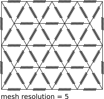 Fig. 1: Triangular section mesh with a resolution of 5 vertices per each long row.
We achieve this globally minimized deformation by simulating the alignment as an elastic system of spring connected vertices. Zero-length springs connect corresponding locations between two overlapping images and warp the images towards perfect overlap. Non-zero length springs within the image preserve each images shape at locally rigid transformation. That way, the system penalizes arbitrary warp and distributes the deformation evenly among all images.
Each image is tessellated into a mesh of regular triangles with each vertex being connected to its neighboring vertices by a spring (see Fig. 1). A triangle of springs has two families of cost minima in the plane: 1) at rigid transformations and 2) at rigid transformations flipped. That is, for all local deformations smaller than the size of a triangle, the mesh will drag towards a rigid transformation. For larger deformation, it may fold. The vertices of a triangle define an affine transformation for all pixels in the triangle.
For those vertices of a source image overlapping a target image, we identify its corresponding location in the target image. The vertex is then connected into the target mesh by a zero-length spring with its target end being located at an arbitrary place in a triangle of the target mesh. This `passive’ end does not contribute to the deformation of the target mesh. During simulation, it moves according to the affine transformation defined by the target triangle. Vice versa, vertices of the target image are connected to their corresponding location in the source image with their `passive’ ends being moved by the respective affine transformation of a source triangle.
Linear Initialization
Both relaxing the system of meshes and identifying corresponding locations between images require good initialization. The former because the meshes will fold otherwise, the latter to narrow the matching space with the benefit of both, increased speed and better reliability. We initialize the system with a linear-per-image optimal pre-alignment based on local image features.1
Block Matching
Corresponding locations are searched through block matching. Initialized from an approximate linear pairwise alignment that is estimated using local image features, the local vicinity around each vertex is inspected for an optimal match. We use the The PMCC coefficent r of a patch around the vertex and the overlapping patch in the other image as the quality measure for a match. The location with maximal r specifies the offset of the vertex relative to the initial linear alignment.
We perform block matching at a reasonably down-scaled version of the images. The ideal scaling factor depends on the application and quality of the signal. To overcome the reduced accuracy of the estimated offset, we use Brown’s method2 to estimate an approximate sub-pixel offset. Furthermore, in order to reject wrong matches, three local filters based on the correlation surface are in place:
minimal threshold for r
if the match has an r lower than a given threshold it is rejected
edge response filter
if the principal curvatures of r(x,y) at matches location are related by a factor larger than a given threshold, the match is rejected for being an edge response.3
ambiguity filter
if the second best r(x,y) is very similar to the best, the match is rejected for being ambiguous. Similar means related by a factor larger than a given threshold.3
See also Test Block Matching Parameters plugin
Parameter Discussion
All parameters that specify a distance in pixels refer to the original scale of the image.
 Fig. 3: Edge response filter. The ratio of the two principal curvatures (Hessian eigenvalues) of at a detection determines how well it is defined in both dimensions. A large ratio signalizes an edge response.
Input
Both plugins work with stacks of images. The stacks might be virtual, which is strongly suggested for very large images.
Output
The plugins export their output as a file or a series of files respectively. In addition, previously extracted local features and feature correspondences are saved for later re-use during parameter triggering (thanks to Albert Cardona for adding this). Make sure that you work in a clear folder when changing the input data because both saved matches and features are identified by their stack index and parameters only.
You can choose whether to interpolate the result or not. Visualize checked will render the spring mesh simulation into a 512×512 pixel stack for demonstration purposes. The result is rendered using a transform mesh similar to the spring mesh discussed above. The parameter resolution specifies the number of vertices in a long row for this mesh, higher numbers give smoother results. Usually, you will never need more than 128. Optionally, the result can be rendered as RGB with green background to explicitly mark empty background pixels e.g. when generating montages for successive series alignment.
Block Matching
Here you specify the scale factor at which matching is performed. Choose this size such that 1) high level noise is effectively invisible, 2) for series alignment such that a pixel is approximately as large as (or larger than) the section thickness. All further distances are specified in pixels of the original image size. The search radius for block matching must include the largest non-linear deformation expected relative to an approximate linear alignment. At the same time it should be kept as small as possible to increase speed and to prevent false matches. Similarly, the block radius should be large enough to include recognizable texture but not too large. Usually, setting both radii to similar values is a good choice. Resolution specifies the number of vertices in a long row of the spring mesh as depicted in Fig. 1. TrakEM2 does not require all image tiles in a montage to have the same size. Therefore, it asks for the side-length of a triangle in the mesh to be specified. That way, the individual mesh resolution for each image can be calculated such that all tiles are modeled by meshes of approximately equal resolution.
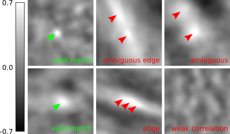
)](/media/filters.jpg) Fig. 4: The effect of block matching filters. (ssTEM image data courtesy of Richard Fetter)
Fig. 4: The effect of block matching filters. (ssTEM image data courtesy of Richard Fetter)
Correlation Filters
The threshold for minimal PMCC r can be higher for montaging (same signal) than for series alignment (changing signal). Higher values will lead to more matches rejected and thus less false positives. The maximal curvature ratio is the threshold for edge responses as depicted in Figs. 2 and 3. The value must be >1.0. Higher values will accept more matches alongside elongated structures and thus lead to potentially more false positives. maximal second best r / best r is the maximal threshold for non-ambiguous detections. Higher values will accept more potentially ambiguous matches that may be false positives.
Local Smoothness Filter
Particularly for series alignment, the local filters based on block correlation will either reject too many matches (false negatives) or let some false matches pass (false positives). Since loosing correct matches will degrade the quality of the alignment, we want to keep the false negatives rate minimal by using only moderate local correlation filters. The remaining false positives can be identified and rejected exploiting the smoothness of the deformation field (Fig. 4). The local smoothness filter inspects each match and compares how well the estimated translational offset agrees with all other matches weighted by their distance to the inspected match. To that end, a local linear transformation (typically rigid) is calculated using weighted least squares. The weight for each match is defined by a Gaussian radial distribution function (RDF) centered at the reference match. A match is rejected if its transfer error relative to the estimated linear transformation is larger than an absolute threshold or larger than k× the average transfer error of all weighted matches (k is specified in the relative field).
Miscellaneous
ImageJ lacking support for alpha-channels, you can choose to ignore perfectly green (rgb:0,255,0) pixels during series alignment. This is a hack to cope with montages not covering the whole canvas. TrakEM2 supports an alpha-channel such that background pixels are automatically treated correctly. Both TrakEM2 and Elastic Stack Alignment offer to consider a series or montage as pre-aligned (checkbox) by which the feature based pre-alignment step can be skipped. For series alignment, the range of layers to be compared can be limited.
Feature Extraction and Geometric Filters
Find documentation at the Feature Extraction page. The approximate transformation model as specified in this dialog is used for geometric consensus filter and pairwise pre-alignment only. It should approximate the actual deformation as closely as possible. That is, you should select an affine transformation in almost any case.
In the montage plugin, all images are compared to each other. This is prohibitive for montages consisting of a large number of images. For large montages, use TrakEM2 where prior information can be used to limit the comparison to overlapping images only. For series alignment, we try to establish matches not only to adjacent section in the series but to as many sections as possible in the previously constrained range (e.g. up to 10 sections). Since the similarity of two section decreases with increasing distance, we can stop matching sections after we have failed to compare closer partners. Still, we want to be able to bridge sections with bad quality or exceptional artifacts. You can specify how many failures you may be willing to bridge.
Optimization
Approximate optimization is used to initialize the alignment for block matching. The iterative optimizer stops latest after maximal iterations but not earlier than maximal plateauwidth even if the square transfer error is not further decreasing, the same parameters need to be specified for spring mesh simulation. Usually, only translation and rigid transformations will result in a reasonable configuration because both similarity and affine transforms have their global optimum at zero-size collapsed state.
For series alignment, springs across sections have a spring constant of 1.0/distance with distance being the absolute index difference in the series. For montage, all springs between overlapping images have a spring constant of 1.0. The constant of springs in the mesh is specified through stiffness. Larger values will result in less deformed, less perfectly aligned results. Very small values may result in unevenly distributed deformation due to premature `relaxation’ of the simulation. You can specify the maximal stretch of springs after which they will disrupt. We have not experimented with this extensively yet.
Future Work
We will further investigate in automatic selection of appropriate parameters depending on available meta-information of the data sets (resolution, section thickness, deformation priors,…). We will investigate appropriate identification strategies for discontinuities in the transformation fields such as section ruptures or folds and cut springs at such places. We will investigate strategies to solve the alignment through hierarchical stages of accuracy for gaining better local accuracy and improved speed.