Foreword
These notes primarily concern the pixel intensity correlation based colocalization methods, where one looks for intensity correlation in different colour channels of individual pixels. Sometimes it is more useful to look for object-based colocalization, where objects are segmented out of images, then objects in different colour channels are tested for spatial overlap: colocalization. In the object-based case, one attempts to acquire images suitable for segmentation. The following principles apply in the case of pixel-based colocalization, but most of the precautions underlined here are general.
Introduction
How can we properly define colocalization? One could suggest:
Degree of overlap between two colour channels in one image, which can be characterised by
- colocalisation coefficients (single global statistics regarding the whole image)
- colocalisation maps (identification of colocalised pixels over the image, spatially)
Estimating colocalisation by looking for yellow colour in images where the green and red images have been colour merged is a bad idea because:
- This is a subjective estimate, depending on how bright the two original images are, and as such is sensitive to manipulation of brightness and contrast of the original images and also incorrect image acquisition (especially saturated/out of detector range images).
- A significant proportion of people are colour blind, and can’t tell the difference between red and green anyway.
- When 2 channel colour merge images are displayed on a computer screen they look different to when they are printed. Green looks brighter than red, and red brighter than blue, because of the way our eyes work. Different printers and different computer screens will give different looking representations of the same 2 channel colour merge image, so it is impossible to be objective about what you see and compre it with what someone else sees.
- There are simple and quick objective methods to estimate colocalisation, so don’t be lazy. You can use them to get hard objective statistics describing the colocalisation in your images, and its easy to do.
- Our brains find color contrast that is not even really there. In the following illusion (Fig. 1), there are only really 3 colors. The “blue”and “green” are exactly the same color: Do not trust your eyes - measure it.
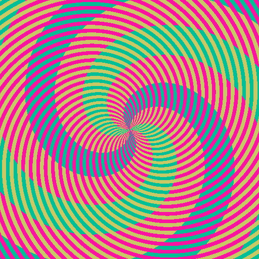 Figure 1: The spirals color illusion
What we need are objective quantitative methods to estimate/measure colocalisation in 2 colour channel images. These will output colocalisation coefficients that should be:
- sensitive to colocalization between one colour channel and the other;
- insensitive to the presence of a non-relevant background;
- insensitive to relative variation of intensities between channels.
But… in order to do quantitative analysis on images, they muse be acquired in the correct way, such that they contain the information that you are tring to measure! You must also understand the limitations of your microscope and the digital imaging process.
Precautions during image analysis
There are various problems that need to be understood and overcome while collecting images at the microscope. No clever analysis can save crappy images (aka. The “crap in - crap out” principle). If you lose or don’t collect information that the microscope could have seen during imaging, it is lost forever. We list here a few of these dangers. Being modest, we should make it clear that some of the difficulties are actually unavoidable and must be lived with, but understood all the same.
Blur
Definition: The Fourier spectrum of the image lacks proper high frequencies.
Definition: The small features/edges of the real object are not well represented in the image.
This phenomenon will artificially enlarge the size of your objects, making them look bigger. The problem with this is that two non colocalizing objects might appear to colocalize in the image because of the blur. This gives false-positive results.
Possible origins of blur are:
- optical system is dirty (objective, sample)
- optical system is misaligned (pinhole, optical components)
- wrong immersion oil / coverslip thickness / immersion medium
- similarly: objective lens correction collars not ajusted
- mechanical drift or moving sample - most apparent with slow imaging
- imaging too deep into the sample ( < 5 µm with oil, > 5 µm with water, > 50 µm with 2-photons system, and you will see spherical aberration due to refractive index mismatch between the objective lens immersion medium and sample)
- widefield microscope system (or on a confocal microscope - optimal pinhole size of 1 Airy Unit not set)
- colorshift: if you don’t know what it is, always use apochromat objectives - these correct for chromatic aberrations (blue bends better than red)
- Inadequate spatial sampling. If your pixels are too big to correctly sample the smallest features visible, you will not see those features.
Some things we can’t do anything about (hey, that’s the light microscopy facility, hum?):
- Diffraction: The spatial resolution of the conventional widefield or confocal (as typically used - noise limited) light microscope is limited by diffraction, and is dependent on the wavelength of the light (shorter is better) and the numerical aperture (NA) of the objective lens (higher is better). XY resolution is better than resolution in Z direction (about 3x better for a high NA objective. Spatial sampling should be done so that there are not less than and not too many more than 2.3 pixels across the resolution limit (according to Nyqvist). For a high NA lens (say a 63x 1.4 oil immersion) this means the pixels in XY should be about 80-100 nm, and in Z about 250 nm. Also see Sampling below.
If the blurring of you images is too much, you might want to consider deconvolution. Have a look at this page from SVI, the guys that provides Huygens software to see how it can help.
Background
Definition: Unspecific signal.
The presence of a high background will generate a huge amount of artificial, irrelevant colocalization. You are not interested in unspecific colocalization - your reviewers might only be mildly happy if you spend a lot of time analysing background. You do not want background to affect your analysis results.
Hopefully our colocalisation analysis methods will be insensitive to small differences in background, but thats no reason not to get it as low as is possible. Having bright real signal and low background improves the “dynamic range” of the information, and thats a very good thing for quantitative analysis.
At the microscope, you must decide what parts of your image are background and not interesting. Then you can set the microscope to give the background very low or zero intensity values in the images.
Getting rid of high background? Consider:
- autofluorescence of the sample / medium / immersion medium (e.g. phenol red)
- staining protocol (bad unspecific antibodies …)
- leaking of excitation light in the emission range, because of inadequate fluorescence filter design
- too low “offset” on a PMT detector in a confocal microscope.
Noise
Definition: Uncertainty of signal.
Colocalisation in a pixel might be false, coming from noise, and thus, not be real. For correlation based statistical approaches to colocalisation analysis, increasing noise lowers the apparent colocalisation. Hence, for noisy images, an attempt must be made to suppress or remove the noise in order to get closer to the true noise free correlation. Constrained iterative deconvolution can act as a smart noise filter that increases contrast and suppresses noise, so widefield and confocal image data should be deconvolved before colocalisation analysis.
Types of Noise:
- dark noise / dark current. False signal with Poisson distribution from thermally generated electrons in the detector. CCD/EMCCD/sCMOS: increases with temperature, so we use cooled cameras, then there is nothing much to do as the noise is then very small and only seen in very long exposures. PMT/Confocal: cooled PMTs help, eg. Leica SP5
- Read noise / digitizer noise / electronic noise from the system (Confocal PMTs get over it with a PMT voltage above about 400). EMCCDs are very sensitive because they amplify a small signal over and above the dark noise and read noise so you can measure it. sCMOS cameras have a very low read noise of an eletron ot two, several times less than a CCD camera.
- Photon shot noise. This is intrinsic statistical noise in the signal coming from fluorescence photons. It follows a Poisson distribution over time, as photons arrive whenever they like at the detector. It’s magnitude is the square root of the number of incident photons measured. So we can increase the “photon signal” to “photon signal noise” ratio by increasing the exposure time or pixel dwell time and collecting more photons, but this contradicts one of the rules to avoid a blurry image - when the sample is moving, and might cause photo bleaching of the dye. On a single point scan confocal microscope it gives a better signal, more photons detected, to do more line scan averages with a pixel dwell time much less than 10 microseconds, than to do one slower scan with more than about 10 microseconds pixel dwell time (this is for complicated photophysics reasons to do with dye dark states, eg triplet state population build up.)
- Amplification noise. The more gain, the more noise. This noise is Gaussian shaped. A solution would be to use lower gains (on a confocal dont use a PMT voltage over about 800, turn the laser power up a bit instead if you can, or do more line scan averaging). On A CCD (especially EM CCD) don’t have the gain too high or you will add noise to your image.
One must have a signal strong enough to allow a good enough signal:noise ratio, or be able to deal with a weak signal and separate it from the noise, using eg iterative deconvolution!
Cross talk and Bleed through
Definition 1: Fluorophores do not match optical components (excitation / emission filters, lasers, dichroics).
Definition 2: You detect emission from the wrong dye, and falsely believe it comes from the right dye.
So… this one is the very worst and most dangerous problem in colocalization experiments. It can be explained with the following spectra:
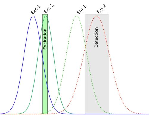
In this picture, the detection setup is configured so as to measure emitted light from the second fluorophore. The problem is that in this detection channel, some of the light emitted by the first fluorophore is also collected and integrated to the channel 2 signal. This is called bleed-through. When you are going to compute colocalization of this channel with the first one, there will be a part of the signal that will colocalize with it whatever it is, since signal coming from the first fluorophore is present in both channels. That is, you generated false-positive result.
You could avoid this by selectively only exciting fluorophore number one, and acquire the first image, then excite the fluorophore number 2 and acquire the second image (sequential imaging). But on these spectra, you can see that the excitation curves also overlap, and that the excitation wavelength hits both dyes efficiently. The two fluorophores will both be excited at this wavelength; a process called cross-talk. Your last hope is that there is a laser line that hits the first excitation spectrum without touching the other, and reciprocally for the second one.
Dye choice is critical here. Avoid DAPI and GFP, since DAPI emission is very broad, and bleeds through into GFP detection. Better to choose a far red nulclear/DMA stain like Draq-5 for use with GFP. Choose dyes by looking at their excitation and emission spectra, and pick dyes that match your microscope fluorescence filters and laser excitation lines (eg. look at the Thermo Fisher Scientific Fluorescence SpectraViewer for doing that). Choose dydters that are well spectrally separated it at all possible. Different microscopes in the LMF have different choices of excitation filter and laser line wavelengths, and different possibilities for emission filters. Choose your dyes carefully.
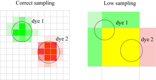
Poor Spatial Sampling
Definition: The pixel size does not allow for a highly spatially resolved colocalisation analysis.
Definition 2: Pixels are too big. Close but separate objects which do not colocalise, appear to colocalise.
As a general rule, you should have each object you image sampled over many pixels. When this is not the case, a colocalization statement cannot be reliable made, as the assumptions of the method no longer hold.
Let’s suppose that you have two objects each with different colour, and you would like to assess if they colocalize in space. If we assume that they don’t colocalise, if the colocalization procedure you are using is working, it should give you a negative result. Consider one molecule of each dye. They are sitting close to each other, but they are not colocalized (in the same place). Now, if the pixel size is so big that these two molecules are imaged on the same pixel, the procedure tells you that they are colocalized. Once again, you are producing false-positive results.
Also remember: since we are doing light microscopy, two objects closer and smaller than the diffraction limit will appear colocalized whatever you do. Particular care must be taken in the case of Z-stack, where the resolution in the Z axis is generally lower than in the XY plane. In order to get around the diffraction limit, and to confirm your colocalisation result, you can do other methods too, such as FRET or FLIM, and immuno precipitation or cellular cofractionation.
Detector Saturation
The problem with “saturated pixels” occurs mainly when we use pixel-based colocalization (i.e. when we are interested in intensity correlation over space). It is possible to derive the quantitative error made with saturation. See here. If pixels/images are saturated (that is having pixels with an intensity level at the top of the range, ie 255 for 8 bit data) then they are missing information about the real spatial intensity distribution in the sample. This is the most important data in your analysis, as you are usually most interested in the brightest objects - right?! That means its a really bad idea to throw that information away when you collect the images.
Chromatic Shift
If the microscope has poor quality or non chromatically corrected objective lenses and / or has other alignment problems, then images of the same object in different colour channels will appear in different places. Even expensive lenses have a little residual chromatic shift. This is very bad, as it means that, especially for smaller objects, you miss some of the real colocalisation. The microscope should be checked with multi colour 1 or 0.5 micron bead samples before imaging to see if there is a significant problem. Images can be corrected for x y and z chromatic shift if a bead image has been taken under identical conditions.
For more details and possible chromatic shift measurement and correction strategies see Chromatic shift origins, measurement and correction
Conclusion
Think about your biological experiment, dyes and imaging, and be careful throughout. Collect image data that is suitable for quantification. For example, Tetraspeck fluorescent beads with 3-4 colors and different sizes (small enough to check shifts) make great positive controls.
Also, for a review of the hardware part, read Zucker, 2006 1.
Credits
From Jan Peychl notes.
The two animated gifs are from the Huygens Software wiki page.
Further reading
The 39 steps: a cautionary tale of quantitative 3-D fluorescence microscopy by J. Pawley 2.