TraJClassifier

Purpose

This Fiji plugin loads trajectories from TrackMate (exported via the action “Export trajectories”), characterize them using TraJ and classificate them into normal diffusion, subdiffusion, confined diffusion and directed/active motion by a random forest approach (through Renjin). It supports local analysis and is therefore able to split a single trajectory into segments with different motion types.

For detailed information please see:

Wagner T, Kroll A, Haramagatti CR, Lipinski HG, Wiemann M (2017) Classification and Segmentation of Nanoparticle Diffusion Trajectories in Cellular Micro Environments. PLOS ONE 12(1): e0170165

Installation

Simply turn on the TraJClassifier update site.

Introduction

Please start by reading the introduction of TraJ, because the TraJClassifier is build upon this library. The TraJClassifier was trained using simulated trajectories of normal diffusion, subdiffusion, confined diffusion and directed motion. For each simulated, we estimated nine features for each trajectory (For more information about these features, go to the TraJ wiki):

• Alpha
• Asymmetry (Asymmetry3)
• Efficiency
• Fractal dimension
• Gaussianity
• Kurtosis
• Mean squared displacement ratio
• Straightness
• Trappedness

These features and the corresponding class were then used to train a random forest classifier. Furthermore the TraJClassifier employs a sliding window to allow local analysis of single trajectories.

As summary, the classification process is as follows:

1. Load trajectories from TrackMate xml file (Exported via the action “Export trajectories”)
2. For each trajectory
   1. Split the trajectory into subtrajectories using a sliding window
   2. Calculate the features of each subtrajectory and classificate them (results are a class l with confidence c for each subtrajectory)
   3. Each position in original trajectory which is contained in a subtrajectory gets a vote for l with the weight c.
   4. Each position in original trajectory gets the class with the majority of votes.
3. Split successive positions with the same class into single segments.
4. Output results

Examples

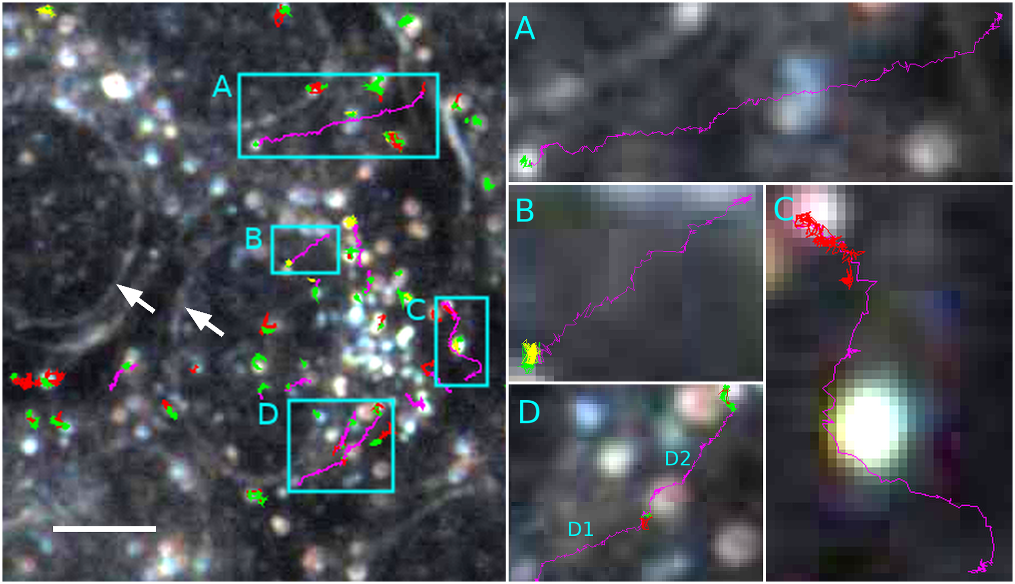
The following figure shows several cells that are gathered within the field of view (left image). While cell borders are not visible in this focal plane, nuclear envelopes stand out clearly under darkfield illumination (white arrows). A total of 246 particle trajectories was identified as either normal diffusion (red), confined diffusion (yellow), anomalous diffusion (green) or directed motion (magenta). Boxed areas (A-D) show selected cases of directed motion:

More examples could be found in

Wagner T, Kroll A, Haramagatti CR, Lipinski HG, Wiemann M (2017) Classification and Segmentation of Nanoparticle Diffusion Trajectories in Cellular Micro Environments. PLOS ONE 12(1): e0170165

Parameters

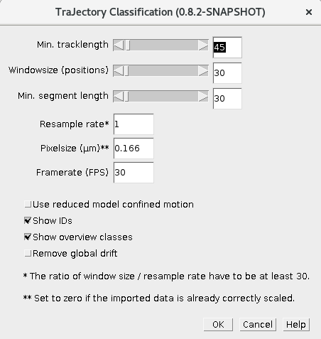
Minimal track length: Minimal number of positions in a trajectory. It has to be greater than the window size. As the window size should be at least 30, the same is true for the minimal track length.

Window size: The parameter determines how many positions are used in the sliding window.

Minimal segment size: After classification of a trajectory it consists of several segments. This parameter determines the minimal segment length. Segments smaller than this length (number of positions) will be removed. It is good rule of thumb to set this parameter to same value as the window size because segments which are smaller than the window size seems to be more error prone.

Resample rate: During the local analysis using a sliding window, one trajectory is split into several subtrajectories. In very noisy cases it could make sense to resample the subtrajectories to increase the signal to noise ratio (e.g. if the rate is set to 2, then only every second position is used in the trajectory). However, we believe that a trajectory should contain at least 30 position therefore the ratio of window size and the resample rate should be >= 30.

Pixel size: Size of a single pixel in µm. However, if your TrackMate data is already scaled, set it to zero.

Frame rate: Frames per second

Use reduced model for confined motion: The shape constants for the confined diffusion MSD model are set to 1.

Show IDs: Show trajectory IDs as overlay. The trajectories IDs given in the format PARENT ID:SEGMENT ID

Show overview classes: Show classes and color codes as overlay.

Remove global drift: In some cases the particles are moving relativ to another object (e.g. particles in a cell). When the object is moving approx. at a constant speed, than it could be possible to estimate it via a global drift estimation and remove this drift component from each trajectory.