Generating and analyzing kymographs with TrackMate

Introduction.

Kymographs are a very useful technique in bioimage analysis, that allow for visually following particles even in data where they are very faint in a noisy background. A moving object drown in noise and background signal could be become barely visible in the source image. In a kymograph its movement often becomes salient, and easier to analyze.

Kymographs rely on a dimensionality reduction that generate a 2D image from a 2D+T or a 3D+T source. They are created by measuring the intensity profile over a line between two fixed points in one time point of the input image. The intensity profile is turned into a 1D line image, and all the 1D line images across all time-points are stacked in the target kymograph. In the 2D image of a kymograph, the time runs along Y from top to bottom, and the space runs along the X dimension and reports the intensity along the line.

The TrackMate-Kymograph extension addresses one issue with the above approach. It is aimed at generating a kymograph between moving points, that we call landmarks in the following. The landmarks that define the kymograph line are simply taken from two tracks in a TrackMate session. The input data can be 2D or 3D. The line would follow a biological structure of interest over time, possibly moving, and we generate a kymograph along this line. To our knowledge, all the other tools that can generate kymographs only work when the line is fixed. The following short documentation shows how to install the plugin and how to use it.

Installation.

The TrackMate-Kymograph extension lives on a dedicated update site, that you need to subscribe to.

In Fiji, launch the updater (Help > Update) and make sure that you have an up-to-date Fiji. When it is done, still in the updater, check the Manage updates sites button. You need to find and check the update site called TrackMate-Kymograph.

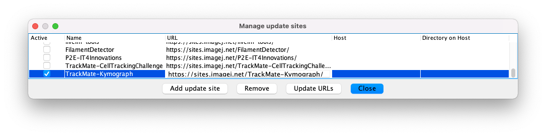
Click OK, and restart Fiji. The extension will appear as a special action in TrackMate.

Creating the landmarks in TrackMate.

We can create a moving kymograph between any two tracks in TrackMate that have at least one time-point in common. So, we just need to create two tracks in the movie we want to generate the kymograph on. This can be done in an automated way if the landmarks have features that could be detected by one of the detectors in TrackMate. Otherwise, we need to add the manually.

The demo dataset.

In the following tutorial, we will use a movie acquired by Dr. Ines Saenz de Santa Maria, in the lab of Pr. Charia Zurzolo, Institut Pasteur. The movie can be downloaded from Zenodo:

Ines follows the transfer of mitochondria through tunneling nanotubes (TNTs) that extend sometimes between two cells.

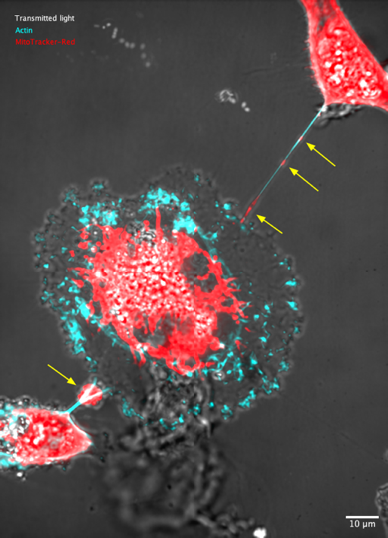
Because the mitochondria appear at small bright structures (yellow arrows above) that travel along a line, kymographs are well suited to analyze their speed. However, the TNT they travel in moves a lot over time, as the cells migrate. The TrackMate-Kymograph extension was built specifically for this application. In the movie used in this tutorial, all the mitochondria are clearly visible. However, one of the key advantage of kymographs is that they allow following very faint structure reliably.

Manually tracking the TNT extremities.

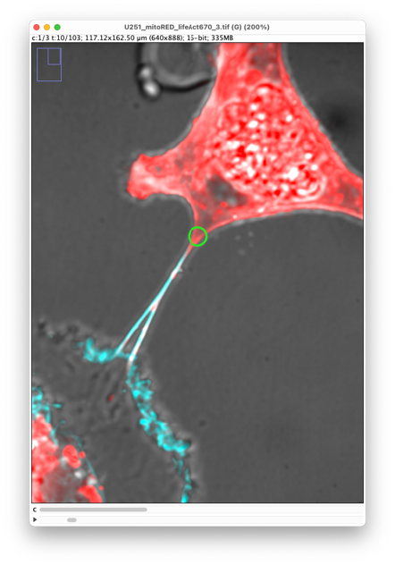
Open the image in Fiji. Its calibration and dimensionality are already setup properly. The first step in the analysis is to create two tracks for the landmarks. They will follow the extremities of the TNT between the central cell and the top-right cell. Because it can be hard to determinate the exact position of the TNT extremity automatically, we will do so manually and use the transmitted light channel as a visual cue.

With the image open, launch the manual tracking version of TrackMate, in Plugins > Tracking > Manual tracking with TrackMate. The TrackMate UI opens, with empty tracking data.

We will now manually create the two tracks for the TNT extremity. The manual editing and creation of tracks is detailed in other tutorials:

• Manual tracking with TrackMate

• Manually editing tracks with TrackMate

But we will repeat here some of the information you can find there.

The source image contains 103 time-points. Manually creating a track over 103 time-points is not so long in TrackMate, but because the cells do not move too briskly, we will accelerate it by creating spots for every 5 time-points, then interpolating in between. There is an option window that helps manual tracking. To make it appear, double click on the TrackMate tool icon in the ImageJ toolbar:

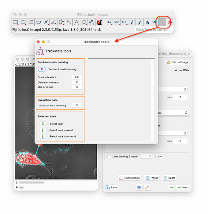
You can see that the Stepwise time browsing setting is already set at 5 time-points. Put this window aside and zoom in the top-right extremity of the TNT. At the beginning of the movie the TNT is wide and filled with dye, which makes it hard to properly define the extremity. Move to the 10th time-point. We suggest using the tip of the triangle formed by the membrane protrusion to define the TNT extremity. We will now add a track that follows this landmark.

With the image active, press ‘Shift+L’ to toggle the auto-linking mode. In this mode, the new spots are automatically linked to the last spot selected, creating, and adding to its track all along. The log panel in the TrackMate tools window should print the message “Toggled auto-linking mode on”.

Position the mouse over the TNT extremity and press ‘A’. A new spot is created at this location. The new spot size is probably too big. With the mouse inside the spot, press ‘Q’ to make it smaller.

Parenthetically:

• Press ‘Shift+Q’ to make it smaller by bigger steps.
• If needed, you can make it bigger by putting the mouse inside the spot and pressing ‘E’ or ‘Shift+E’.
• If you need to move the spot to fix its position after creation, put the mouse inside it, press and hold the ‘Space’ key and move the mouse. The spot will follow the mouse location.
• If you want to delete a spot, move the mouse inside it and press the ‘D’ key.

Notice that the spot we just created is selected. It is highlighted in green and painted with a thick line. Because we toggled the auto-linking mode, the next spot we will create will be automatically linked to this one. To select a spot, click in it.

Now we want to create the next spot in the track by jumping 5 time-points ahead. The shortcut to do that is ‘G’. Use ‘F’ to move back by 5 time-points. The number of time-points to jump over by using ‘F’ and ‘G’ is set in the Stepwise time browsing in the TrackMate tools window. (In our case, even if we start from the time-point 10, it will jump to the time-point 11, because TrackMate jumps by 5 time-points intervals, measured from the first time-point, so that you always fall on time-points 1, 6, 11, 16, etc. This is not an issue for us.)

In this new time-point, create a new spot over the TNT extremity by pressing ‘A’ over its location. The log window should state that it added a new spot to this time-point and created a link with the previous spot. The last spot you created becomes selected.

Press again ‘G’ to jump ahead in time and continue creating spots at the TNT extremity until the end of the movie. You should create a track that follows the TNT extremity in a short time:

We now must do the same, but for the other TNT extremity. It is important to do it with another track. So, to avoid adding spots corresponding to the TNT lower-left extremity to the other extremity track, press ‘Shift-L’ again to toggle the auto-linking mode off.

Move back to time-point 10, zoom to the lower-left extremity, and add the first spot. The TNT has a branching there that will later fuse. We will first generate a kymograph for the lower branch. As visual cue, we suggest picking the protrusion edge:

Press ‘Shift-L’ again to toggle the auto-linking mode on and repeat the manual tracking procedure with the ‘A’ and ‘G’ keys we used for the other extremity.

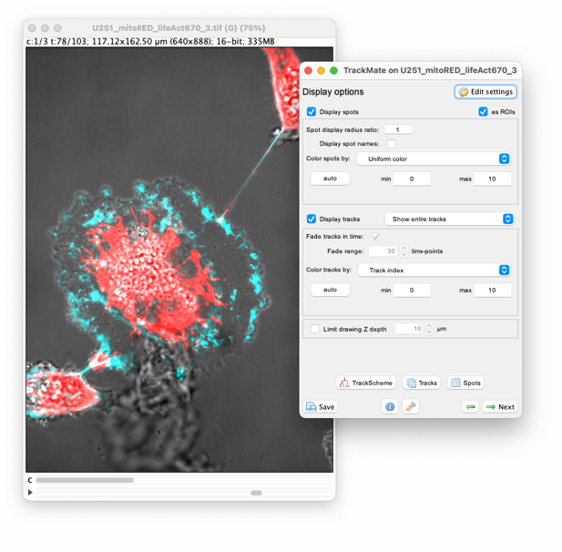
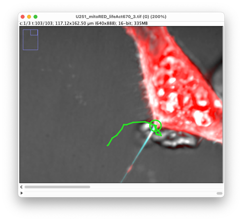
We now have two tracks, one for each extremity. But the spots are present only one every 5 frames. We need to interpolate to fill the gaps. To do so, move to the last panel of the TrackMate UI, by clicking on the Next button twice in the main panel. In the action list, find the one called ‘Close gaps by introducing new spots’.

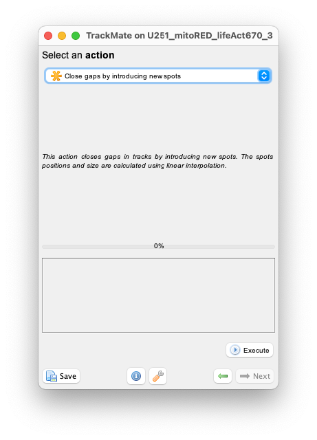
Run it by pressing ‘Execute’ button. The tracks have now one spot per time-point.

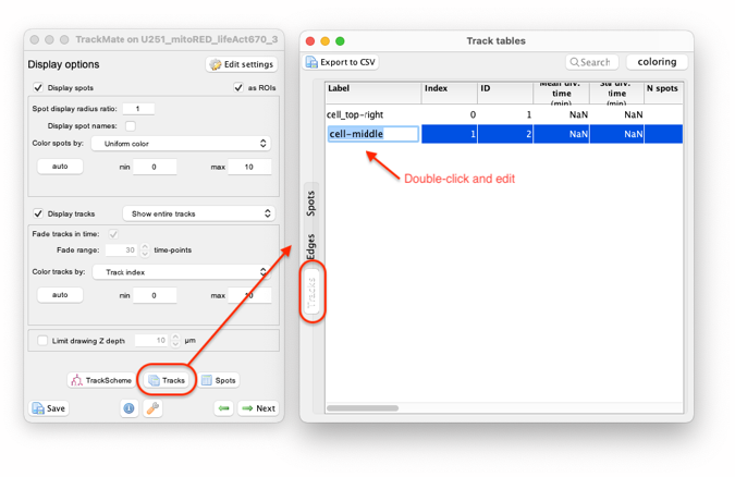
This is not mandatory, but we can also rename the tracks to remind us of what landmark they follow. One of the ways to do so is to use the track table that can be generated from the display option panel:

It is a good idea to save the TrackMate file now, by pressing the ‘Save’ button now.

Generating the kymographs.

The TrackMate file we just created by saving contains only the tracks of the landmarks. This part was not specific to kymographs, it is the general way TrackMate performs manual tracking. We will now use these tracks to generating moving kymographs.

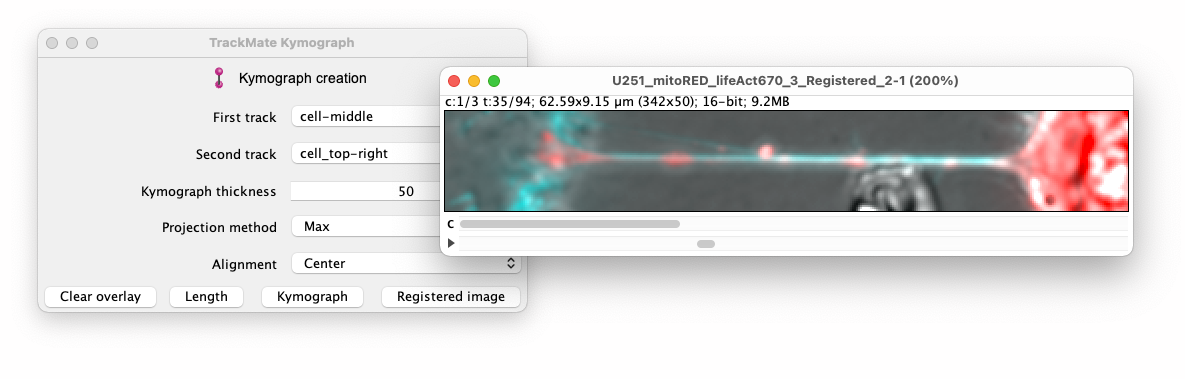
In the main TrackMate window, move again to the last panel, dedicated to actions. If you installed the TrackMate-Kymograph extension properly, a new action should appear, called ‘Moving kymograph’. Press ‘Execute’ to make its panel appear:

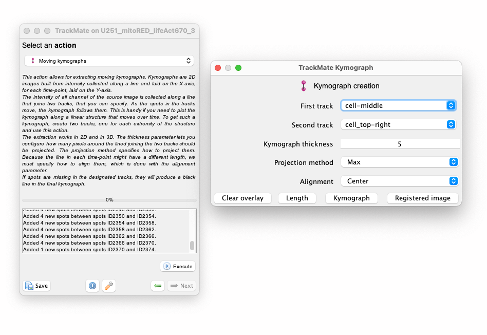
The option panel is very simple. You mut specify the tracks for the two landmarks. In our case since we only have two tracks there is no choice there. When you have multiple cells with many landmarks, it is useful to have the tracks renamed to identify them easily.

The ‘Kymograph thickness’ sets how far pixels can be to be included in the intensity measurements. For instance, with a thickness of 5 pixels, the intensity at one point in the kymograph will be taken 2.5 pixels away from the kymograph line, orthogonally to it, and in both directions.

The ‘Projection method’ allows specifying how to compute the kymograph intensities from these multiple pixels. The ‘Max’ projection method will take the pixel with the largest intensity. The ‘Mean’ projection method will take their average.

The ‘Alignment’ method let you specify how the kymograph should be aligned. Since the landmarks move, the kymograph lines will not be of constant length. We still need to align them and there are different ways. ‘Center’ will keep the center of the kymograph line fixed. ‘First track’ and ‘Second track’ will flush the lines to the left and the right respectively. This is important when computing velocities later. The velocities measured from the kymograph will be calculated with respect to this fixed point.

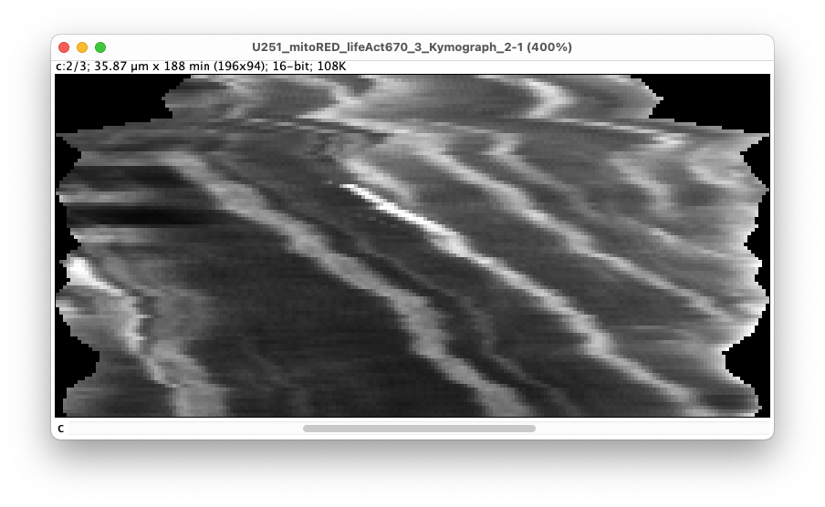
Finally, several buttons offer to generate different outputs. We are first interested in generating kymographs, so press the ‘Kymograph’ button. This window should appear: The image that appears is the kymograph. Time runs along the Y dimension, from top to bottom.

The space dimension runs along X. The left border corresponds to the first track used as landmark, and the right to the second one. We do not have the same unit nor dimension in X and Y. In the image window header, we can read the images size: 35.87 µm x 188 min (196x94). Recent version of ImageJ allows specifying different units for the X and Y axis. As we will extract the speed from the slope of stripes in this image, it is important that the units are right. With the settings used above, the left part corresponds to the middle cell and the right part corresponds to the top cell. Single mitochondria appear as thick lines that run close to a diagonal in the kymograph image. Because they go from left to right and top to bottom, we can conclude that the mitochondria transfer from the middle cell to the top cell in this movie. If the lines would be vertical, it would mean the mitochondria are not moving. If the lines are close to horizontal, it means that the mitochondria move at a very high speed. The slope of these lines is linked to the object speed, which will be used by the analysis part of this tool.

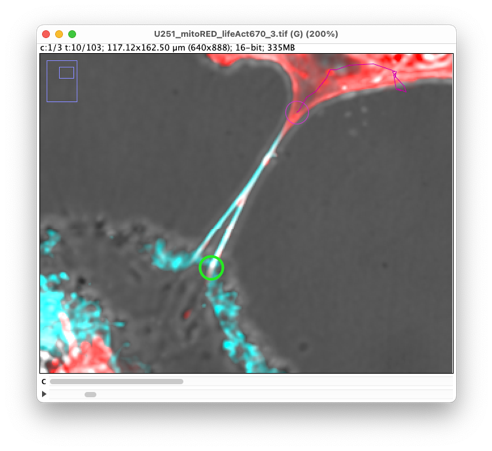
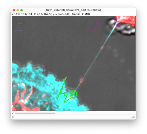
The kymograph image is displayed in grayscale and is a multi-channel image (one channel per channel in the source image). The second channel is the one for the mitochondria, and this is the one we need to analyze. We notice some dark stripes in early time-points. We can understand where they come from if we inspect the source image. The kymograph line along with its thickness is represented by a yellow rotated rectangle. It shows what pixels are used to generate the kymograph. Initially, the TNT is bent, and the kymograph line misses its middle, which results in the dark stripes we see above. We can fix this by increasing the ‘Kymograph thickness’ setting above, setting it for instance to 15:

(Close the other kymograph images and their respective controllers.) The new kymograph now shows a new bright line appearing roughly at the middle of the Y axis. This is a mitochondrion from the other TNT branch (the upper one) fusing with the main branch. To include mitochondria from the two branches we could use a much larger thickness, which we won’t be doing here.

Analyzing the kymographs.

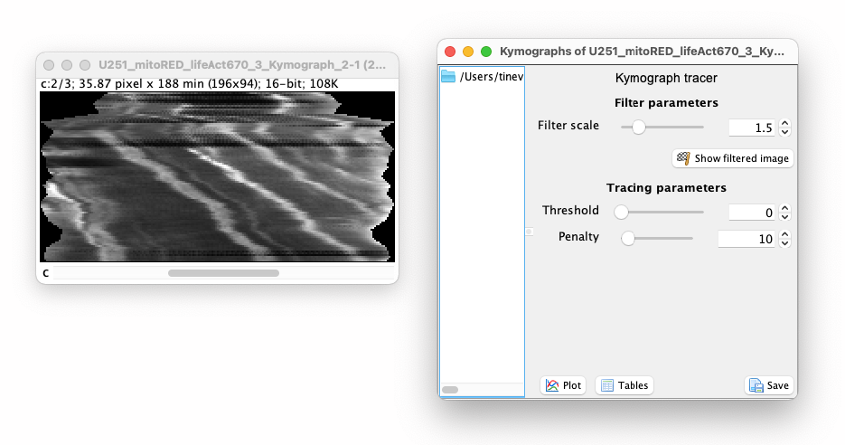
You could save the kymograph image and analyze it with another tool. (For instance, the Kymograph-Tracker of Icy: https://icy.bioimageanalysis.org/plugin/kymographtracker/.) The controller window, called ‘Kymograph tracer’, that appeared next to the image allows for performing a basic analysis, that we will describe here. We won’t be using the TrackMate window, nor the kymograph creation window we described above. You can close them or put them aside for now.

In the Kymograph tracer window, there is a ‘Save’ button at the bottom right. Use it to save the kymograph now. This creates a JSON file, which is a text file following a specific format:

{  	
 	"name": "~/DemoDataset/U251_mitoRED_lifeAct670_3_Kymograph_2-1.tif",  
 	"spaceInterval": 0.1830000292800047,  
	"timeInterval": 2.0,  
	"spaceUnits": "µm",  
	"timeUnits": "min", 
	"kymographs": []  
} 

Right now, it is almost empty since we did not create a kymograph yet. It only contains the path to the kymograph image (which was saved along with the JSON file), and the units and pixel sizes.

Tracing kymographs.

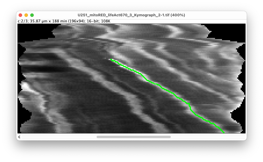
Let’s create the first kymograph. Move to the second channel of the kymograph image to show the mitochondria channel. We will start by tracing the kymograph for the brightest mitochondrion. It starts roughly in the middle of the image around x = 14.5 µm, y = 60 min. (It appears at this later time and this position because it comes from another TNT. We only see it first when the mitochondrion enters the 15-pixel wide box around the line we follow.) To trace it:

• Click once on the beginning of the trace. In the controller the message ‘Starting a new kymograph’ appears.
• Move the mouse (without clicking) downwards in the image, roughly following the trace. The automatic tracer only follows traces from top to bottom (forward in time). By pressing the ‘Shift’ key, the trace found will be shown in cyan.

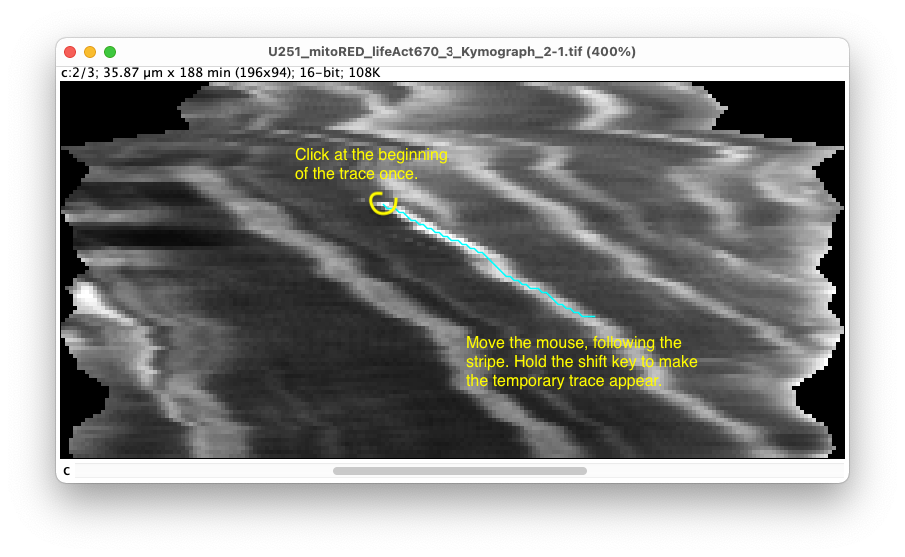
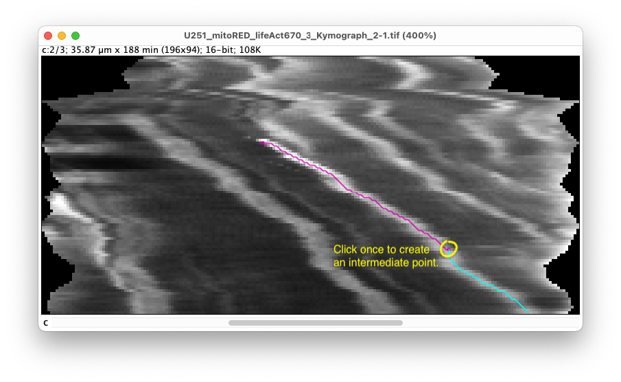
If the trace deviates too much from the bright stripe, click on an intermediate point. The trace between the start and this point is now fixed, and a new automatic tracing starts from the intermediate point. In the controller, the message ‘Added segment to kymograph’ appears.

• When you are finished with the stripe, double-click at the end point to finish editing the trace and store it. In the controller, the message ‘Finished kymograph’ appears.

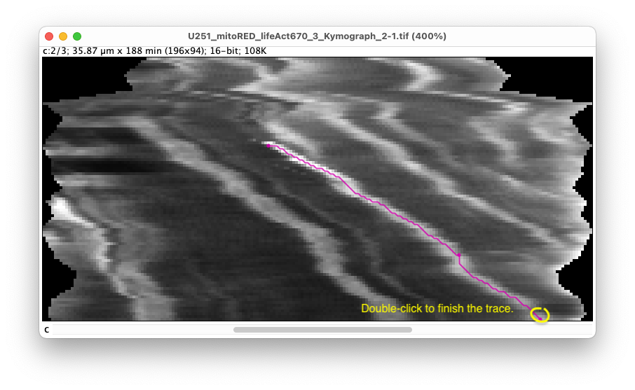
It also shows in the left sidebar that we have now a new kymograph called ‘Kymograph_1’ made of two segments. The name of the kymograph and of the segments can be modified by double clicking on their label in the sidebar. They can also be removed by with the delete key, but careful, there is no undo/redo, and a missing segment in the middle of a kymograph might results in incorrect results.

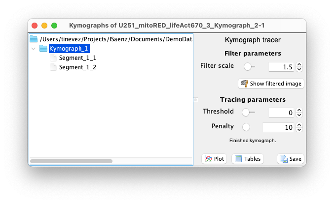
Automated tracing parameters.

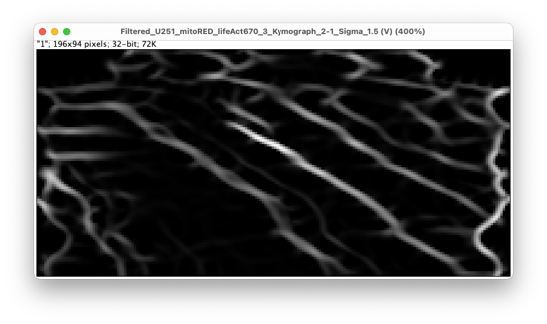
The automated tracing algorithm is based on the A-star path searching algorithm¹. The path searching is performed on a filtered version of the image, using the Tubeness filter² to stress ridges. You can set the scale of this filter using the slider next to the ‘Filter scale’ parameter in the controller. This value should be set to be approximately the width, in pixels, of the stripe you want to trace. By clicking on the ‘Show filtered image’ you can see what is the resulting of the filtering. The automated tracer follows continuous bright structures in this filtered image.

The tracer can be further configured with the ‘Threshold’ and ‘Penalty’ settings:

• The threshold value sets a value below which pixels are ignored for tracing. It ranges from 0 to 1, with 1 representing the maximal pixel value in the image.
• The penalty sets the “strength” of intensity versus the shortest distance. A strong value (max is 100) will force the path to stick to pixel with high values, at the cost of having a path that is irregular. Setting the penalty to 0 makes the automatic tracer completely ignores the pixel values and create paths that are simply the shortest path between the starting and ending points.

In our experience, the default values (0 and 10) are good enough to start with.

Getting the tables and plots.

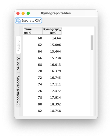
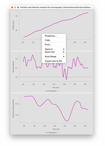
Once you finished tracing the kymograph of interests (and saving them), you can get the numerical data out of them. The ‘Tables’ button will create a new window in which the kymograph data is shown. There are tables in this window. The first one is for the position of the kymographs, the second is for the velocity and the third one for the smoothed velocity. The position and velocity values are already smoothed and interpolated by splines, to avoid jagged data points since the tracer sticks to pixels. The smoothed velocity dataset includes a supplemental smoothing step using LOESS interpolation³ if there are enough data points, and no extra smoothing otherwise. Each table has a ‘Export to CSV’ button that will export the currently active table to a CSV file.

The ‘Plot’ button generates a window where the plot of these 3 datasets. The plots have basic controls and can be exported by using a popup menu shown by right-clicking on the plot you want to modify or export.

Analyzing the registered movie.

The kymograph tracing, we have been using above is a great tool to detect and quantify the movement of weakly labeled objects. When they are bright and clear, a more direct approach is to track them in the moving frame of the kymograph line. Close the kymograph tracer controller and window and focus back to the main TrackMate Kymograph action window. Next to the ‘Kymograph’ button, the ‘Registered image’ button will generate such an image. To better capture the context around the TNT, it is a good idea to increase the ’Kymograph thickness’ parameter to for instance 50:

This new image is a time-lapse movie with the same calibration that of the source. It cuts 2D planes from the (possibly 3D) source image, that follow the kymograph line defined by the two tracks you specified. It can be saved and used as input to classical analysis or tracking using e.g., TrackMate. The positions and velocities measured in such a movie will be with respect to the moving frame of the first or second track points, or their center, as set by the ‘Alignment’ parameter in the controller. The ‘Projection method’ parameter is ignored.

Other features.

On the same controller, the ‘Clear overlay’ button will remove the yellow box painted in the source image that shows what is included in the kymograph or registered image after pressing the ‘Kymograph’ or ‘Registered image’ buttons.

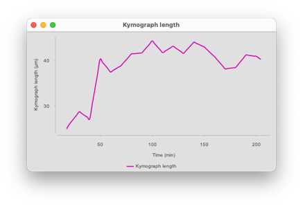
The ‘Length’ button will generate a plot of the distance between the two tracks over time.

Footnotes