The SLIM Curve plugin for ImageJ has been discontinued in favor of FLIMJ.
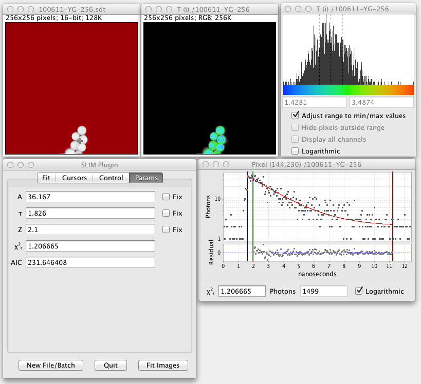
SLIM Curve screenshot
SLIM Curve is an exponential curve fitting library used for Fluorescent Lifetime Imaging (FLIM) and Spectral Lifetime Imaging (SLIM). It was developed by Paul Barber and the Advanced Technology Group at the Cancer Research UK and Medical Research Council Oxford Institute for Radiation Oncology, as well as the Laboratory for Optical and Computational Instrumentation at the University of Wisconsin-Madison. SLIM Curve was used for FLIM functionality in the Advanced Technology Group’s Time Resolved Imaging (TRI2) software, as well as in the SLIM Curve plugin for ImageJ.
There are two algorithms used for curve fitting within SLIM Curve:
- The first is a triple integral method that does a very fast estimate of a single exponential lifetime component.
- The second is a Levenberg-Marquardt algorithm or LMA that uses an iterative, least-squares-minimization approach to generate a fit. This works with single, double and triple exponential models, as well as stretched exponential.
The SLIM Curve library code is written in C89 compatible C and is thread-safe for fitting multiple pixels concurrently. Several files are provided as wrappers to call the library from Java code: EcfWrapper.c and .h provide a subset of function calls used by the SLIM Curve plugin for ImageJ, these may be invoked directly from Java using JNA. In addition there is a Java CurveFitter project that provides a wrapper to the SLIM Curve code. This invokes the C code using JNI, with loci_curvefitter_SLIMCurveFitter.c and .h.
Installation
The SLIM Curve plugin is available from the “SLIM-Curve” update site.
Once you have installed the SLIM Curve plugin it becomes available on the menu under Analyze › Lifetime › SLIM Curve.
Usage
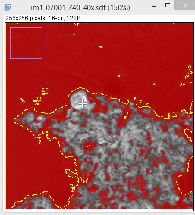
When you run the plugin you will first be prompted to load a lifetime data file. (This should have a .sdt or .ics suffix.) Once the file loads a grayscale version of the lifetime image pops up, produced by summing the photon counts for all time bins for each pixel:
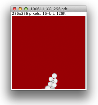
Here the red color signifies pixels that have a low photon count and will be excluded from any fitted images that are produced. The threshold value for this is adjustable in the user interface. When fitted images are created, yellow pixels signify fitting errors. During analysis of fitted images, blue pixels indicate outliers.
The crosshair cursor shows the current fitted pixel. This starts out as the brightest pixel in the image. Clicking around the grayscale image fits other pixels.
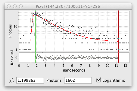
The fitted decay graph pops up showing the results of the pixel fit:
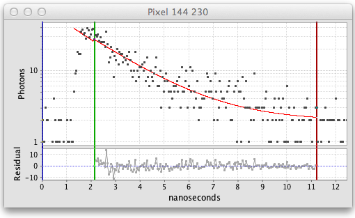
Here the graph shows black squares for the observed photon counts over time and a red line for the fitted curve. There are also vertical blue, green, and red lines or cursors that mark the region of the decay being fitted. Below the decay graph is a graph showing the Residuals, the difference between the observed and fitted values. For a good fit the residuals should have a low value range and exhibit a random pattern.
The user interface panel also pops up, allowing you to control the settings of the fit. On the initial tab of the user interface panel entitled Fit you can choose what kind of fit and analysis you want to perform:
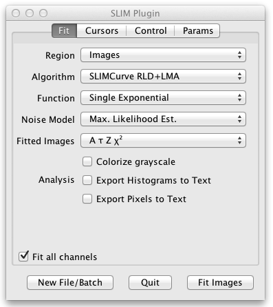
- Region allows you to fit the entire image, a single pixel, the sum of all pixels, or the sum of each ROI defined on the grayscale image.
- Algorithm selects the fit algorithm. SLIMCurve RLD+LMA is recommended. This uses a rapid lifetime determination (also known as a triple integral fit) to quickly estimate the fitted parameters. Then a Levenberg-Marquardt least-squares fit is done to refine those estimates.
- Function lets you choose between single, double, and triple exponential fitted components. The stretched exponential fit can be used to characterize the distribution of multiple exponential lifetime components.
- Noise Model compensates for the noise in the fitted data. The recommendation here is to use the Maximum Likelihood Estimation noise model. This compensates for low photon counts.
- Fitted Images selects what output images are produced when you fit the entire image. These output images are colorized using a special lifetime LUT (lookup table or palette). You may select A the intensity, Tau the lifetime, Z the background, and/or the ChiSquare for each pixel of the fit. When you are fitting multiple exponential components you may also select f the fractional contribution and F the fractional intensity, as well as Tm the mean of the fitted taus. For stretched exponential fits you may select H which characterizes the distribution of the multiple lifetimes.
- Colorize grayscale is an option to combine the LUT colors indicating the parameter values for each pixel with the grayscale image.
- Analysis lets you optionally specify further analysis of the fitted results: Export to Text produces a text file of the fitted values. VisAD sends the fitted data to a VisAD plugin for further analysis. Display Fit Results produces a single image containing all the output images.
- The Fit all channels checkbox selects whether to fit all channels or just the current channel when the source image has multiple channels.
The next tab is entitled Cursors:
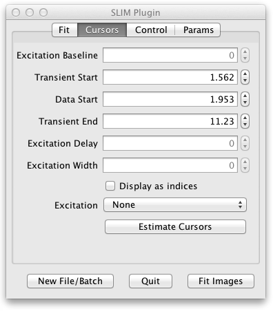
Here the positions of the fit cursors are listed. There are two kinds of cursors:
The transient cursors bracket which region of the decay to fit. Transient Start corresponds to the blue vertical line at the left of the Fitted Decay Graph. Data Start is the green line in the middle. Transient End is the red line at the right. Dragging these cursor lines on the Fitted Decay Graph will also change the values on the Cursors tab of the UI and cause a refit of the current pixel.
The excitation cursors bracket which region of the excitation or instrument response function decay to use in the fit. If an excitation is loaded the decay is shown in an Instrument Response Function graph with cursor lines similar to the Fitted Decay Graph:
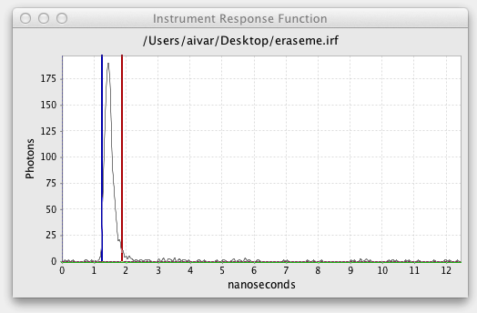
The horizontal green line controls the Excitation Baseline, the minimum photon count to be included in the excitation. The vertical blue and green cursor lines define the start and end of the excitation. The Excitation Delay is the offset between the Transient Start and the start of the excitation. Excitation Width is the end of the excitation minus the start.
The cursor values are represented as time values (except for Excitation Baseline which is a photon count) for compatibility with TRI2, but the checkbox lets you see the corresponding exact indices into the decay histogram.
The Estimate Cursors button resets the cursors, estimated for the current pixel transient and excitation. They can also be tweaked by dragging the cursors or entering new values. If the tweaking doesn’t optimize the fit you can return to the original settings with the Estimate Cursors button. If you load a new image none of the settings change, so you may want to use Estimate Cursors to find cursors more appropriate for the new image.
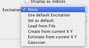
The Excitation dropdown is used to create, load, or cancel an excitation. Using an excitation is optional but makes for a better fit. Typically the experimenter will create a separate excitation image with the same setup but only imaging some non-fluorescent material such as beads.
To create an excitation is currently a two step process. Run SLIM Curve with the excitation lifetime image, then find a suitable pixel to use, perhaps the default, brightest one. From this tab of the UI under Excitation select Use Current X Y. The program will prompt for a name and place to save the excitation file. For the second step use the New Image/Batch button to load the lifetime image you want to analyze. Now select Load from File in the Excitation dropdown and enter the file name you saved. When an excitation is loaded the cursors are estimated.
If an excitation is loaded it is also shown on the fitted decay graph in light gray:
In the next tab of the UI panel titled Control you can fine tune some aspects of the fit:
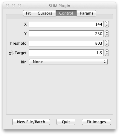
- X and Y specify the location of the last single fitted pixel. (You can fit a single pixel by setting Region to Single Pixel and clicking the Fit Pixel button or by just clicking on the grayscale image.)
- Start and Stop select the starting and ending time bins to be fitted.
- Threshold determines the minimum number of photons in the decay curve for a given pixel that are needed in order to fit that pixel.
- ChiSquare target controls the value of chi square at which the iterative LMA fitting process will stop. (Fitting also stops after a maximum number of iterations.)
- Bin can compensate for lower photon counts at the expense of some spatial resolution by binning the photons from adjacent pixels.
The final tab of the user interface panel is a section entitled Parameters which displays and lets you constrain the fitted parameters. The actual contents of this subpanel will depend upon the Function selected.
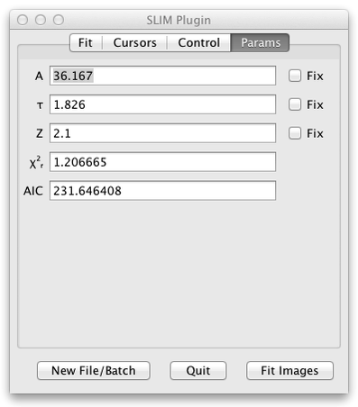
For each parameter:
- A label, such as A1 or Tau2 identifies the parameter.
- A textfield shows the current value of that parameter.
- A checkbox labelled Fix lets you fix the value of that parameter during the fit.
- Both the reduced chisquare and the AIC are measures of the goodness of fit. AIC stands for the Akaike Information Criterion. Unlike chisquare AIC has no absolute meaning, but can be used to compare single, double, and triple exponential fits to determine which model has the best fit.
After fitting a single pixel or all of the pixels summed the fitted parameters can be viewed in this user interface panel Params section.
SLIM Curve starts up with the Region under the Fit tab of the UI set to Image. Pressing the Fit Image button will cause the images selected in the Fitted Images drop down menu item to be generated. The list of images in the Fitted Images drop down menu varies with the fitting Function selected, i.e. single or multiple exponential. It includes combinations of the fitted params that show up in the Params tab of the UI, as well as fractional contribution, fractional intensity, and tau mean for multi-exponential fits.
When a fitted image is created a histogram tool panel also pops up. This panel shows the range of values encountered in the fitted image and the LUT used to display those values, as well as a histogram of the distribution of those values in the image.
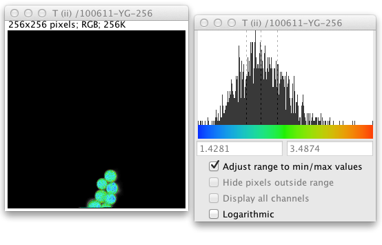
By default the histogram tool comes up in automatic mode, the start and end of the LUT range automatically adjust to the minimum and maximum values in the image, so you can see the distribution all of the fitted values. Here the dashed gray lines indicate the quartiles of the distribution. If you uncheck this Adjust range to min/max values checkbox the histogram will zoom in based on the quartile range. (This uses Tukey’s Outlier Rule: If Q1 is the first quartile value and Q3 the third, let the interquartile range IQR equal Q3 - Q1. Then values less than Q1 - 1.5 * IQR or greater than Q3 + 1.5 * IQR are considered outliers and are discarded.) You can also either enter new start and end values (this is useful to impose a uniform LUT range so you can compare different lifetime images) or just drag markers at the start and end of the histogram.
Outlier pixels will display as black pixels. If you put the cursor over them in the fitted image the fitted value will show up in the ImageJ toolbar. The Hide pixels outside range checkbox discards these outliers, they are excluded from all fitted images and histograms, they display as black, and the fitted value becomes Double.NaN. This special value is excluded from any subsequent statistical measurements on the fitted image. They also show up on the grayscale image in blue.
For images that have more than one channel, there will also be a checkbox to Display all channels. When you display all channels the histogram displays values for all channels combined. Lastly the Logarithmic checkbox shows the histogram graph as logarithmic values. Note that this histogram tool is enhanced to always show at least a one pixel bar graph in non-logarithmic mode if the value is non-zero so that outliers can be seen. Similarly in logarithmic mode it shows a proportionate bar graph if the histogram bin count is one so that bin counts of 1 and 0 can be distinguished.
Save/Load default excitation
Controlling the default excitation
As loading/saving excitation file is something user need to do every time, the process has been simplified. Whatever macro user wants to set as default excitation, user should load the sdt file normally, set transient start/end time and save the file as *irf file. Then from the drop down user should select “Set as default”. This way, the excitation with the transient start/end time is saved as default excitation. Later, when needed to load the default excitation, selecting “Use default excitation” will load the default one.
Macro language support
All the operations in SLIM Plugin operation are completely compatible with the popular ImageJ macro language. Each of the button, selection, choice of algorithm, binning, noise model, default excitation selection with custom start-end time is completely macro record-able. Below is a typical macro recording for a typical usage where the user sets the algorithm, noise model, changes transient time, loads default excitation, sets the chi2 target, fixes A value for fitting and then starts fitting.
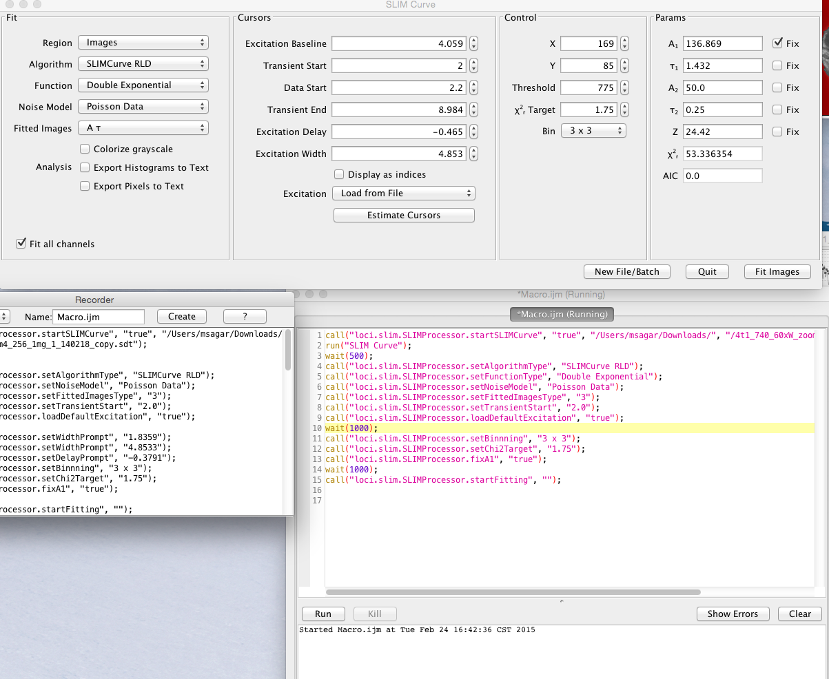
Example of macro recording SLIM Curve
The list of commands are as follows:
-
Start the plugin with a lifetime(*.sdt or *.ics) file:
call("loci.slim.SLIMProcessor.startSLIMCurve", "true", "/Users/msagar/downloads/", "/4t1_740_60xW_zoom4_256_1mg_1_140218_copy.sdt"); run("SLIM Curve"); -
Change the algorithm:
call("loci.slim.SLIMProcessor.setAlgorithmType", "SLIMCurve RLD"); -
Set number of components of exponents:
call("loci.slim.SLIMProcessor.setFunctionType", "Double Exponential"); -
Change noise model:
call("loci.slim.SLIMProcessor.setNoiseModel", "Poisson Data"); -
Change which parameters for fitting:
call("loci.slim.SLIMProcessor.setFittedImagesType", "3"); -
Set transient start time:
call("loci.slim.SLIMProcessor.setTransientStart", "2.0"); -
Set the binning:
call("loci.slim.SLIMProcessor.setBinnning", "3 x 3"); -
Load default excitation:
call("loci.slim.SLIMProcessor.loadDefaultExcitation", "true"); -
Load default excitation:
call("loci.slim.SLIMProcessor.loadDefaultExcitation", "true"); -
Set the chi2 target value:
call("loci.slim.SLIMProcessor.setChi2Target", "1.75"); -
Fix the A value(All “fix” are recordable):
call("loci.slim.SLIMProcessor.fixA1", "true"); -
Start fitting:
call("loci.slim.SLIMProcessor.startFitting", ""); -
Loading an existing excitation file:
call("loci.slim.SLIMProcessor.setExcitation", "/Users/msagar/Documents/qwe.irf"); -
Set to double exponential (no of component =2):
call("loci.slim.SLIMProcessor.setFunctionType", "Double Exponential"); -
Fix Z for double exponential fitting:
call("loci.slim.SLIMProcessor.fixZ", "true");
For batch processing, the whole operation can be recorded. Macro record the name of the files needed for exporting the values. A typical batch processing macro code looks like the following:
-
Start fitting:
call("loci.slim.SLIMProcessor.batchModeSet", "true");
call("loci.slim.SLIMProcessor.exportFileSet", "pixel.tsv", "histograms.tsv", "summary.tsv");
call("loci.slim.SLIMProcessor.startBatchMacro", "");
When “Export Histogram to Text” or/and “Export Pixels to Text” is selected for exporting the output to a CSV or TSV file that is also recorded in macro. A typical code looks like this:
call("loci.slim.SLIMProcessor.exportHistoFileName", "histoGram.csv", ",");
call("loci.slim.SLIMProcessor.exportPixelFileName", "pixel.csv", ",");
call("loci.slim.SLIMProcessor.setAnalysisList", "true", "2");
Complete Macro Example
Complete macro example with exporting histograms and pixel information to CSV file:
call("loci.slim.SLIMProcessor.startSLIMCurve", "true", "/Users/msagar/downloads/", "/4t1_740_60xW_zoom4_256_1mg_1_140218_copy.sdt");
run("SLIM Curve");
call("loci.slim.SLIMProcessor.setFunctionType", "Double Exponential");
call("loci.slim.SLIMProcessor.loadDefaultExcitation", "true");
wait(1000);
call("loci.slim.SLIMProcessor.setWidthPrompt", "1.8359");
call("loci.slim.SLIMProcessor.setWidthPrompt", "4.8533");
call("loci.slim.SLIMProcessor.setDelayPrompt", "-0.3791");
call("loci.slim.SLIMProcessor.setBinnning", "3 x 3");
call("loci.slim.SLIMProcessor.fixZ", "true");
wait(1000);
call("loci.slim.SLIMProcessor.startFitting", "");
call("loci.slim.SLIMProcessor.exportHistoFileName", "histogram1.csv", ",");
call("loci.slim.SLIMProcessor.exportPixelFileName", "pixel1.csv", ",");
call("loci.slim.SLIMProcessor.setAnalysisList", "true", "2");
Batch mode
Once you are satisfied with the fitting settings for a source image you can use those same settings on a series of similar images. All images should have the same number of time bins. To get into batch mode merely click on the New File/Batch button and select a folder or a selection of images. The batch mode UI will pop up:
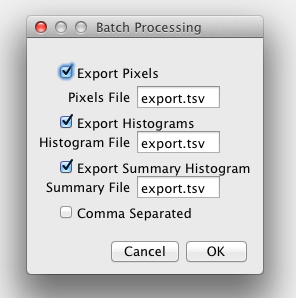
You can export the pixel values, histogram values and statistics, and summary histogram values and statistics to a text file. This can be the same file or separate files. The default is tab separated values but the checkbox allows comma separated values.
Once the batch processing starts a window will pop up showing the histogram and statistics for each lifetime file, as well as a summary histogram and statistics:
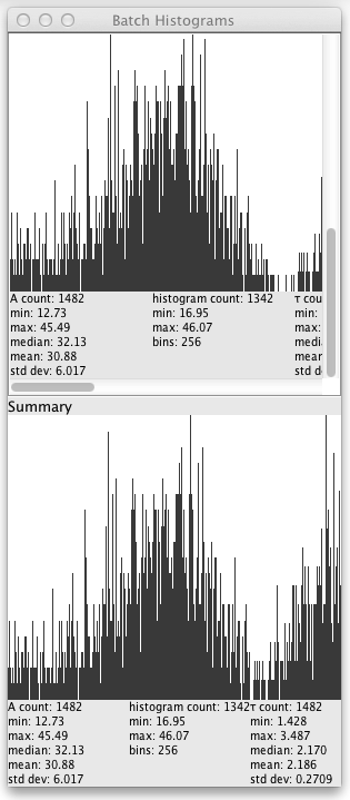
Each source lifetime image has a row of histograms for each of the parameters in the Fitted Images dropdown of the Fit tab of the UI. Clicking on the row loads the source image into the plugin.
Note that you can’t start out in batch mode, you need to fit a single image first and make sure the fitting settings are appropriate.
Example macro
dir = getDirectory("Choose Source Directory ");
Dialog.create("Batch Processing");
Dialog.addCheckbox("Export Pixels to Text", true);
Dialog.addCheckbox("Export Histograms to Text", true);
Dialog.addCheckbox("Export Batch Histogram to Text", true);
Dialog.addString("Save as", "", 20);
Dialog.show();
pixels = Dialog.getCheckbox();
histos = Dialog.getCheckbox();
batchHisto = Dialog.getCheckbox();
output = Dialog.getString();
if (pixels || histos) {
    list = getFileList(dir);
    setBatchMode(true);
    okay = call("loci.slim.SLIM_PlugIn.startBatch");
//  if (okay) { // doesn't work
        for (i = 0; i < list.length; i++) {
            showProgress(i+1, list.length);
            call("loci.slim.SLIM_PlugIn.batch", dir + list[i], output, pixels, histos);
        }
        call("loci.slim.SLIM_PlugIn.endBatch");
//  }
}
if (batchHisto) {
    list = getFileList(dir);
    setBatchMode(true);
    call("loci.slim.SLIM_PlugIn.startBatchHisto");
    for (i = 0; i < list.length; ++i) {
        showProgress(i+1, list.length);
        call("loci.slim.SLIM_PlugIn.batchHisto", dir + list[i], output);
    }
    call("loci.slim.SLIM_PlugIn.endBatchHisto");
}
Segmentation using classification
For some specific applications, you might want to analyze a specific segment in the lifetime image. In particular, Fiji’s Trainable Weka Segmentation plugin is very useful for machine learning based segmentation. We can train the classifier with one image with certain training instances, then use that classifier to segment additional images. With segmented data, we can create a mask and using the ROI manager we can overlay the ROI to analyze different part of the image. The steps for segmentation using classification are:
- Open a lifetime image using the SLIM Curve plugin.
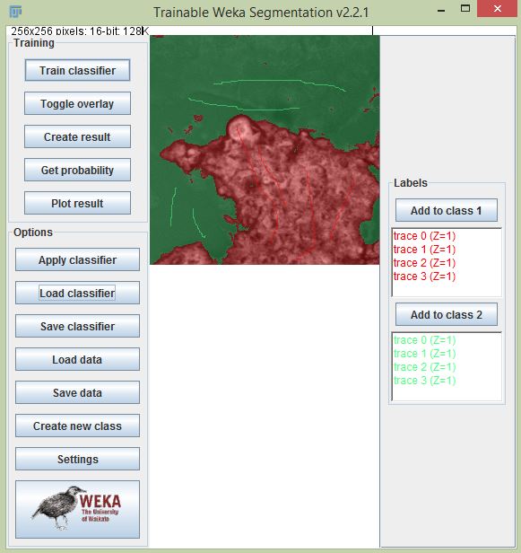
- Train the classifier using Trainable Weka Segmentation.
- Create instances to train your classifier with the number of classes required.
- Train classifier by clicking the “Train classifier” button.
- Select “Create result” to create the segmented image (you can save the classifier to use it later).
- Use the Thresholding tool to threshold the image to remove the region not needed.
- Run the Create Mask and Create Selection commands to make the ROI. You can execute commands easily using the search bar (press L).
- Add the ROI to ROI manager by pressing T. Use it on overlay with lifetime image and start analyzing.
Result comparison
The result of the SLIM Curve plugin compares reasonably with standard lifetime analysis software like SPCImage. Here is a small comparison between the lifetime obtained with SPCImage and SLIM Curve for lifetime analysis of coumarin 6 dye. The lifetime image which has been analysed can be found here and the urea image that is used to create the excitation can be found here. The excitation was set between 1.5 to 5.2 ns. And the shift(Z) was fixed at 0.7. A one component fit was performed. Binning was 3x3. The results shows that the lifetime values obtained from SLIM Curve varies between 0.5%-2% from the value obtained from SPCImage for 5 points selected randomly. The lifetimes are given below for the same locations are given below.
| X | Y | SLIM Curve(in ps) | SPCImage(in ps) | Difference(%) |
|---|---|---|---|---|
| 166 | 113 | 2582 | 2567 | 0.584 |
| 93 | 37 | 2488 | 2539 | -2.01 |
| 195 | 76 | 2548 | 2602 | -2.08 |
| 207 | 202 | 2464 | 2487 | -0.92 |
| 219 | 49 | 2470 | 2493 | -0.922 |
Getting help
If you have questions, please ask on the Image.sc Forum with the slim-curve tag.