Parallel Iterative Deconvolution

Purpose

Parallel Iterative Deconvolution is an ImageJ plugin for iterative deblurring. This plugin takes advantage of multi-core processors.

Documentation

The plugin code is based on a MATLAB toolbox: RestoreTools by James G. Nagy and several of his students, including Julianne Chung, Katrina Palmer, Lisa Perrone, and Ryan Wright and also on Iterative Deconvolve 3D by Robert Dougherty.

It implements the 4 following iterative methods:

• MRNSD - Modified Residual Norm Steepest Descent
• WPL - Wiener Filter Preconditioned Landweber
• CGLS - Conjugate Gradient for Least Squares
• HyBR - Hybrid Bidiagonalization Regularization

Please refer to the website for details and examples.

Introduction

What is Deconvolution?

In applications such as astronomy, medicine, physics and biology, scientists use digital images to record and analyze results from experiments. Environmental effects and imperfections in the imaging system can cause the recorded images to be degraded by blurring and noise. Image deconvolution (sometimes known as image deblurring) is the process of reconstructing or estimating the true image from the degraded one. Image deblurring algorithms can be classified into two classes: spectral filtering methods and iterative methods. Other classification divides the algorithms into methods that do not require any information about the blur (also called blind deconvolution) and the methods that need that information. The information about the blur is usually given in the form of a point spread function (PSF). A PSF is an image that describes the response of an imaging system to a point object. A theoretical PSF can be obtained based on the optical properties of the imaging system. The main advantage of this approach is that the obtained PSF is noise-free. The experimental technique, on the other hand, relies on taking a picture of a point object, for example a distant star. In this work we assume that the PSF is known and given in the form of an image.

What is Parallel Iterative Deconvolution?

With iterative deconvolution methods, a sequence of approximations is constructed, where hopefully subsequent approximations provide better reconstructions. Mathematically this is equivalent to solving a particular optimization problem involving a PSF and a blurred image, which could be formulated as something simple like a least squares problem, or something more complicated that incorporates (possibly nonlinear) constraints. As with spectral filtering methods, regularization must be incorporated using, for example, a priori constraints, or through appropriate convergence criteria, or even a combination of such techniques. Well known examples of iterative image reconstruction algorithms include expectation maximization (EM) type approaches (such as the Richardson-Lucy algorithm), conjugate gradient (CG) type methods, and many others. One important advantage of using iterative algorithms is that they can be used on a much wider class of blurring models, including spatially variant blurs. Although iterative methods are generally more expensive than spectral filtering methods for simple spatially invariant blurs, they are much more efficient for difficult spatially variant blurs. Moreover, it is possible to incorporate constraints (e.g., nonnegativity) in the algorithms. The challenges in iterative algorithms concern the regularization (how to stabilize the iterative method in the presence of noise), and determination of an appropriate stopping iteration.

Parallel Iterative Deconvolution is an ImageJ plugin for iterative image deblurring. The code is derived from RestoreTools: An Object Oriented MATLAB Package for Image Restoration written by James G. Nagy and several of his students, including Julianne Chung, Katrina Palmer, Lisa Perrone, and Ryan Wright and also from Iterative Deconvolve 3D written by Robert Dougherty. The current version implements four iterative algorithms: Modified Residual Norm Steepest Descent (MRNSD), Wiener Filter Preconditioned Landweber (WPL), Conjugate Gradient for Least Squares (CGLS) and Hybrid Bidiagonalization Regularization (HyBR). Although the plugin can handle arbitrary-sized 2- and 3-dimensional images, its usage is limited to grayscale images. To deconvolve a color image, you would have to split the channels and deblur each channel separately.

How to use

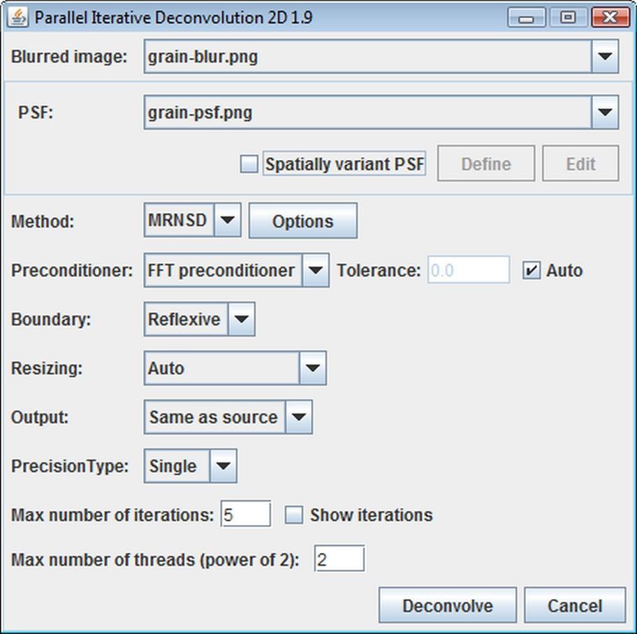
There are eight drop-down lists (combo-boxes) available in the GUI. From the Blurred image list, you can choose a blurred image. PSF list is for selection of a point spread function image. The content of these two lists depends on what is currently open in ImageJ - if no image windows are displayed then both lists are empty. The next two lists (Method and Preconditioner) allow you to select an algorithm used for deconvolution (MRNSD, WPL, CGLS, HyBR) and a preconditioner. The preconditioner is used for speeding up the convergence (so that you will get a better reconstruction after fewer iterations). Currently only the fast Fourier transform-based preconditioner is available (WPL uses the Wiener Filter as a preconditioner). The tolerance for the preconditioner is computed automatically by default (Auto check-box), but it is also possible to specify the value manually. In the Boundary combo-box you can choose from three types of boundary conditions: Reflexive, Periodic and Zero. The first ones are usually the best choice. The Resizing combo-box allows you to specify how the blurred image will be padded before processing. The Minimal resizing means that the pixel data in each dimension of a blurred image are padded by the size of the corresponding dimension of a PSF image. If the Next power of two option is selected, then the pixel data in each dimension of a blurred image are padded to the next power-of-two size that is greater or equal to the size of an image obtained by minimal padding. Finally, the Auto option chooses between the two other options to maximize the performance. The Output list is used to specify the type of an output (reconstructed image) and in the Precision combo-box you can choose a floating-point precision used in computations. Practice shows that a single precision is sufficient for most problems.

There are few other important options in the GUI that require some explanation. The Max number of iterations text field is used to specify how many iterations a given method should perform. It is a maximal value, which means that the process of reconstruction may stop earlier (when the stopping criterion is met). When the Show iterations check-box is selected, then the reconstructed image will be displayed after each iteration. Finally, in the Max number of threads (power of 2) text field you can enter how many computational threads will be used. By default this value is equal to the number of CPUs available on your machine.

The Options button (next to the Method combo-box) is used to display a dialog window with advanced preferences for each algorithm. All of these options are described in the following subsections.

MRNSD Options

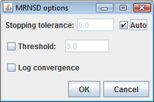
MRNSD has only three advanced properties. The Stopping tolerance text field allows you to manually specify the value that will be used as a stopping criterion. By default that value is computed automatically. When the Threshold option is enabled, then all values in the reconstructed image that are less than the value specified in the threshold text field are replaced by zero. However, since MRNSD is a nonnegatively constrained algorithm, this option is not very useful and is disabled by default. Finally, selecting Log convergence effects in displaying the record of the convergence in a separate Log window.

WPL Options

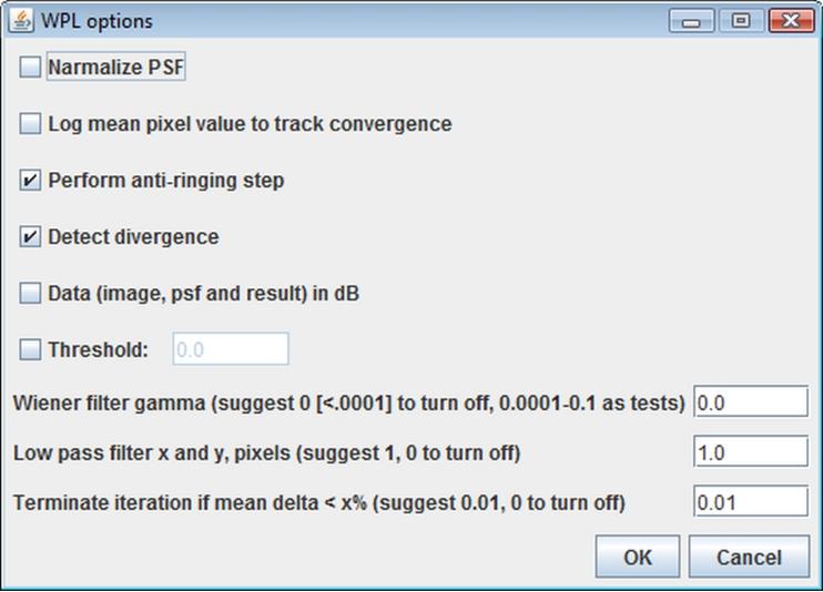
WPL, similarly to MRNSD, is a nonnegatively constrained algorithm, therefore the Threshold option is also disabled by default. Moreover, the Log mean pixel value to track convergence has the same functionality as in the case of MRNSD - the record of the convergence is displayed in the separate Log window. If Normalize PSF is selected then the point spread function is normalized before processing. To reduce artifacts from features near the boundary of the imaging volume you should use the Perform anti-ringing step option. The Detect divergence property stops the iteration if the changes appear to be increasing. You may try to increase the low pass filter size if this problem occurs. For WPL, the inputs in decibels are permitted (Data (image, psf and result) in dB). This is uncommon in optical image processing, but is the norm in acoustics. The Wiener filter gamma is a tolerance for the preconditioner. It is intended to speed up the convergence, but can produce spurious artifacts. Setting this parameter to zero turns off the preconditioner (Wiener Filter). The Low pass filter x and y settings, in pixels, provide a way to smooth the results and accelerate convergence. Choose 0 to disable this function. Finally, the Terminate iteration if mean delta less than x% is used as a stopping criterion.

CGLS Options

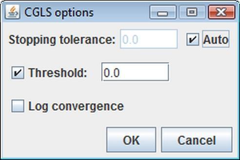
CGLS options panel looks exactly the same as the MRNSD options panel. The only difference is that the Threshold option is enabled by default, since it is not a nonnegativity constrained method.

HyBR Options

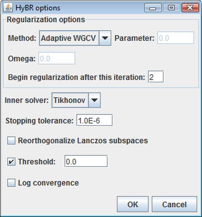
To understand all the details about advanced properties of HyBR you should first read this paper. In the HyBR options panel the properties relevant to regularization are grouped in the box called Regularization options. The Method combo-box allows you to decide how the regularization parameter will be computed. If you select None, then the value of the parameter has to entered in the Parameter text field. When WGCV (Weighted Generalized Cross-Validation) is chosen then you have to specify the weight (Omega) manually. In the Begin regularization after this iteration text field you can decide after which iteration the regularization will begin. Before that iteration the QR factorization is used to solve the least squares problem.

Besides regularization properties, you can adjust five other options. In the Inner solver combo-box you can choose the solver that will be used at each iteration. Currently it can be either Tikhonov or None. If None is selected as an inner solver, then the QR factorization is used to solve the least squares problem. In the Stopping tolerance text field you can enter a value that will be used to detect flatness in the GCV curve as a stopping criteria. If Reorthogonalize Lanczos subspaces is selected, then during the process of Lanczos bidiagonalization, the subspaces will be reorthogonalized. Usually this is not required, so by default this option is unused. The Threshold check-box should be selected, because HyBR does not compute a nonnegative solution. The Log Convergence has the same functionality as for all other methods.

Spatially Variant PSF

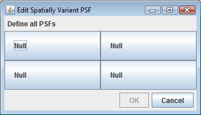
There are three elements in the GUI that have not been described above, namely: Spatially variant PSF check-box, Define and Edit buttons. These controls allow you to work with spatially variant PSFs (i.e. if you have multiple PSF images associated with a single blurred image). Fig. In the Create Spatially Variant PSF panel you can specify the number of PSFs in the form of 2D (or 3D) matrix. Then, after clicking OK button, the Edit Spatially Variant PSF panel will appear. This dialog contains a grid of buttons that you can use to enter paths to the PSF files.

How to Obtain a Theoretical PSF?

There are several ImageJ plugins for generating a theoretical point spread function:

• PSF Tool for ImageJ by the ETH Computationnal Biophysics Lab
• Diffraction PSF 3D by Robert Dougherty
• Deconvolution3D by Pierre Besson.

To use these tools you need to know some parameters of your microscope setup and sample like NA, RI of mounting medium, wavelength, etc.

2D Spatially Invariant Example

After opening the image to deconvolve and the image of the PSF, start Plugins › Deconvolution › 2D Iterative Deconvolution…

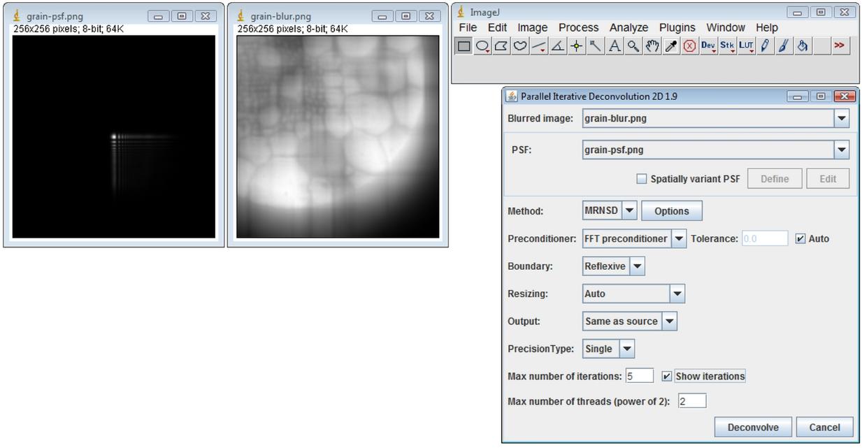
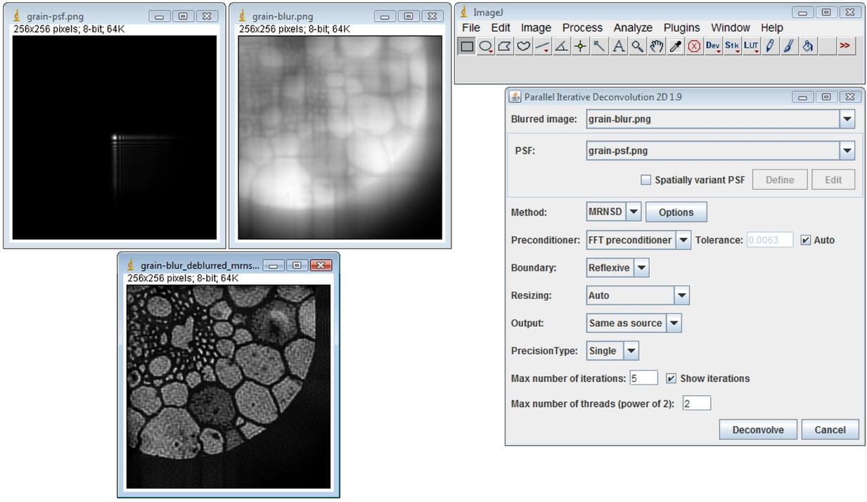
Clicking on the Deconvolve button results in this:

2D Spatially Variant Example

After opening the image to deconvolve, start Plugins › Deconvolution › 2D Iterative Deconvolution…, select Spatially variant PSF check-box and click on the Define button

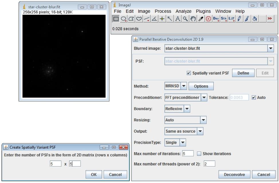
Enter 5 x 5 and click OK button in the Create Spatially Variant PSF panel, then in the Edit Spatially Variant PSF panel you have to define all 25 PSFs

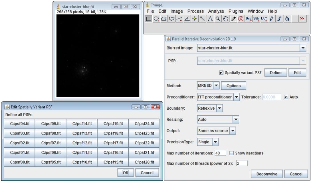
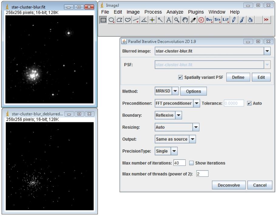
Enter 40 in the Max number of iterations text field and click on the Deconvolve button. You have to adjust the color balance of both images (Image › Adjust › Color Balance…>Auto from Fiji menu).

3D Spatially Invariant Example

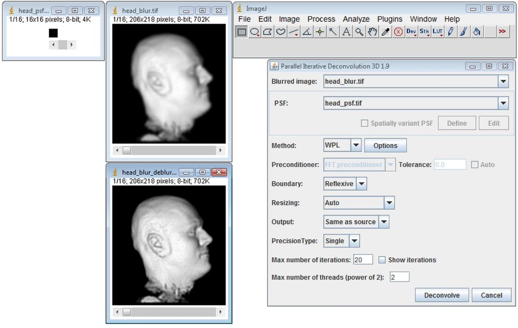
After opening the image to deconvolve and the image of the PSF, start Plugins › Deconvolution › 3D Iterative Deconvolution…

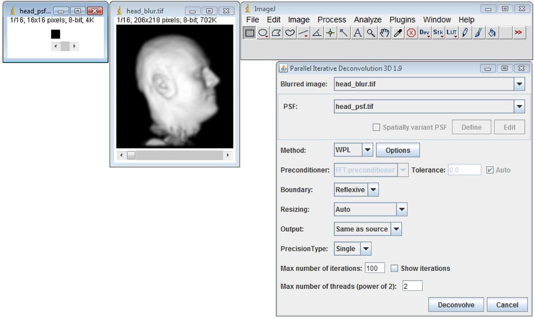
Choose WPL method, click on the Options button and set all the properties as shown below

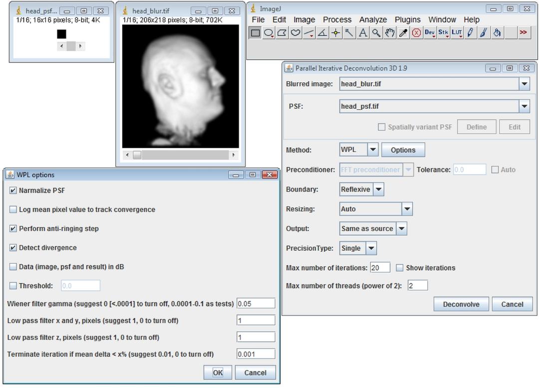
Enter 20 in the Max number of iterations text field and click on the Deconvolve button

See also

• Parallel Spectral Deconvolution by the same author, for another set of methods.

Version history

• 1.0: January 30, 2008
  • Initial release.

• 1.1: February 5, 2008
  • Fixed bug in PSFMatrix_2D causing IndexOutOfBoundException.
  • Added Benchmark_2D.

• 1.2: February 15, 2008
  • Added single precision.
  • Added 3D algorithms.
  • Added exceptions handling.

• 1.2.1: February 16, 2008
  • Fixed bug causing IllegalArgumentException in vectorize().

• 1.2.2: February 19, 2008
  • Fixed bug causing IllegalArgumentException in getFft3().

• 1.3: February 24, 2008
  • The overlap-save algorithm for invariant multiplication was replaced by the non-blocking version in PSFMatrix_2D and PSFMatrix_3D.
  • Fixed bug in MRNSD (division by zero).

• 1.4: March 4. 2008
  • Added threshold option.
  • Added options panel for MRNSD and CGLS.
  • Changed the title of a deblurred image.
  • Memory optimization in HyBR.

• 1.5: March 10, 2008
  • Fixed bug causing improper refreshing of combo boxes holding the list of open images.
  • From now on Deconvolve and Cancel buttons are disabled while deconvolution is in progress.
  • From now on the main GUI window cannot be closed by using the button from the title bar.

• 1.6: April 18, 2008
  • The plugin is updated to use Parallel Colt 0.4.

• 1.7: August 26, 2008
  • New method: Nonnegatively Constrained Gauss-Seidel.
  • Added support for macros.
  • Optimization in MRNSD.
  • Added javadoc distribution.
  • Bzip2 is used to compress tar archives.
  • The plugin is updated to use Parallel Colt 0.5.

• 1.8: November 21, 2008
  • Added resizing option (no need to pad the image to the next power-of-two size).
  • Added output option (a deblurred image is automatically converted to the chosen type).
  • NNGS has been renamed to WPL - Wiener Filter Preconditioned Landweber.
  • The plugin is updated to use Parallel Colt 0.6.

• 1.9: April 11, 2009
  • Added IterativeDeconvolver interface and abstract classes for 2D and 3D iterative algorithms.
  • Non-preconditioned and preconditioned algorithms have been merged.
  • Fixed bug causing NullPointerExceptinon when a blurred image or a PSF was renamed.
  • Refactoring and cosmetic changes.
  • The plugin is updated to use Parallel Colt 0.7.2.