Colocalization by Cross Correlation
This plugin attempts to determine: the average distance between non-randomly spatially associated particles, the standard deviation of that distance (which should also reflect the width of the PSF in the image for diffraction limited images), and two statistical measures of the association. It does this by performing a cross-correlation function (CCF) between the two images, operating in a similar manner to Van Steensel’s CCF except this plugin performs the CCF in all directions and provides additional information, such as the standard deviation and statistical measures. It currently works on 2D/3D single-channel images, supports time-series analysis, and requires a mask of all possible localizations for the signal in one of the images.
Installing the Plugin:
Available on the list of ImageJ updates sites. Requires Fiji.
How to use Colocalization by Cross Correlation (CCC):
Brief overview
- Correct for chromatic shift
- Prepare a mask of the region to be analyzed
- Deconvolve the images (Optional but recommended)
- Convert images to 32-bit (Image > Type > 32-bit)
- Measure and subtract the mean background for both images (Process > Math > Subtract)
- Verify accurate scaling (Image > Properties)
- Run the plugin
Prepare a mask for the pixel randomization
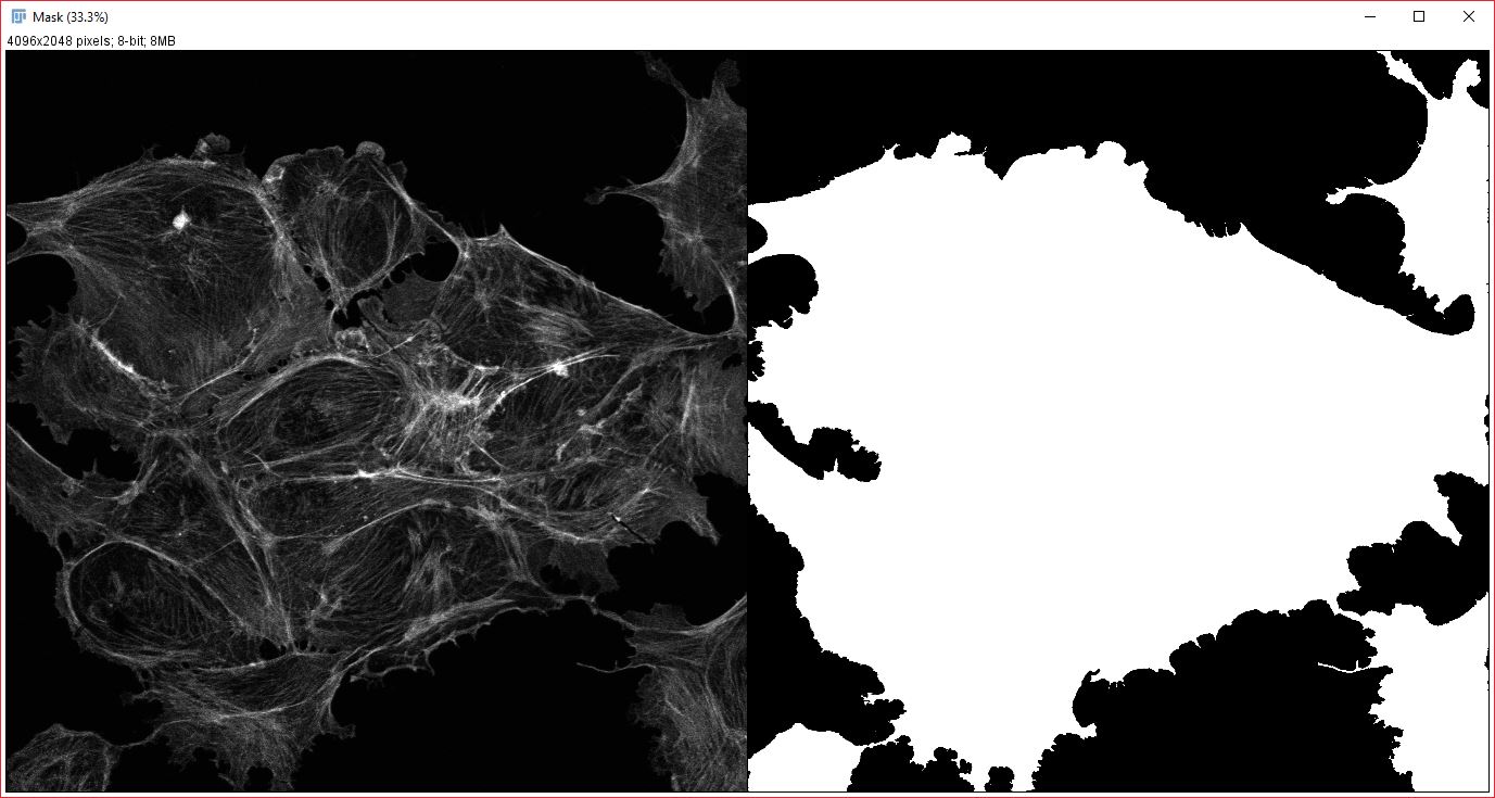
Analysis mask: An example of an appropriate mask for analyzing cross-correlation of cytoplasmic proteins(right), generated from an actin stain (left).
To get the best possible results, you will want to create and save a segmented mask for one of your images. This should be a mask of where within the image your want to search for spatial correlations. Generally, the mask should contain all possible localizations for your stains or dyes, or it should be a mask of localization for your null hypothesis (i.e if you hypothesize a protein is localized to the mitochondria, you would want your mask to encompass the entire cell). As an example, say you are studying correlation between two nuclear proteins, then you would want your mask to cover the nucles, which could be created easily using a DAPI or Hoechst stain (the mask itself does not need to be generated from either image your are trying to correlate). If you were studying cytoplasmic proteins, you would want your mask to cover the entire cytoplasm. The mask is very important and not using it could easily lead to undesired correlations. This is because without a mask this plugin will find correlations at any distance, and, if say you are studying nuclear proteins, can easily correlate one nuclei to the nuclei of a neighboring cell (cells are often highly repetitive and spaced relatively evenly). This broad correlation is the low spatial frequency component, and if not corrected for your results will be affected by it. However, when an appropriate mask is used, these cell to cell correlations will be subtracted out during the analysis.
Prepare your images
Deconvolving your input images can drastically improve the results of CCC and is highly recommended.
It’s also best to use an appropriate background subtraction method on the two data images in order to lower the background pixel values. While pixels outside of the masked region do not contribute to the cross-correlation result, having a high signal to background ratio within the masked region will help improve the confidence signifiantly. Images should be converted to 32-bit depth prior to background subtraction. This should be done to allow negative values in the image, which will improve the results of the statistical measure. After converting to 32-bit, the mean background value, measured from a region devoid of signal, should be subtracted from the image. For 3D images where the majority of voxels are background, you can use the search bar to run the ‘stats.median’ ops function, which will give you an appropriate background value for the entire image.
Additionally, the images (particularly 3D) need to be correctly scaled (Image > Properties), otherwise all axes will be assumed to have the same scale and your mean correlation distance will be in pixels.
Run the plugin
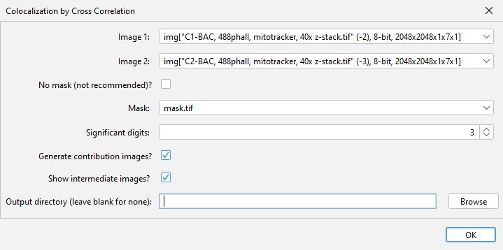 The plugin can be found in the Analyze > Colocalization menu after it has been installed. At the dialog menu, select the two images and the analysis mask to be used. If the possible localizations for your dye/stain encompasses the entire image, you can check the no mask box instead. The plugin can also calculate what signal within each input image contributed to the result by checking the “Generate contriubtion images” checkbox. This process does use more memory, so should be disabled if an out of memory error message is received. A multiple term sum-of-Gaussians curve can be optionally fit to the data by setting the “Number of Gaussians to fit” to 2 or more (discussed below). If the “Show intermediate images” box is checked, the plugin will open images showing the cross-correlation images, both before and after subtraction of the low spatial frequency component. This can be useful for understanding the function of the plugin, or for visualizing the direction of the correlation if your sample has a polarized axis. More details on the contribution and intermediate images can be found below.
Citing CCC
- A. McCall, (2024) Colocalization by cross-correlation, a new method of colocalization suited for super-resolution microscopy. BMC Bioinformatics
Interpreting the results:
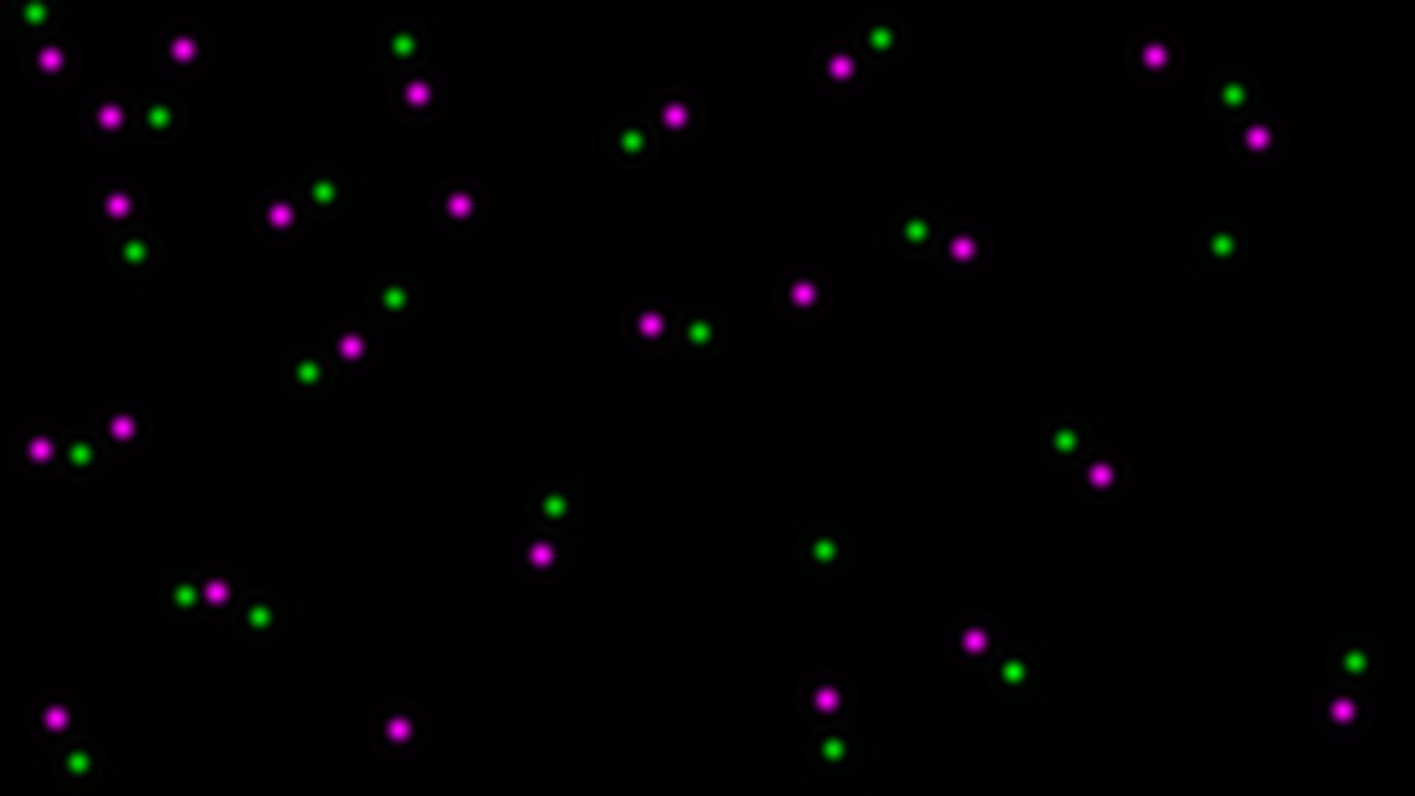
To help describe the results, we will use the simple, idealized example shown below. This example analyzes the cross-correlation of two 2D images composed of equally sized spots (shown as a composite image). Most of these spots are paired to spots of the other channel at a set distance, however some are not at this distance or are not paired. We can see from the results that the strongly correlated spots are approximately 3.28 µm apart, with a standard deviation of ~0.6 µm. The contribution image highlights the spots that are within this correlational distance of each other, while suppressing the spots that are outside this range. We used correlation at a distance for this example to highlight one of the strengths of this technique, but this can be done for traditional “colocalized” images that have a mean cross-correlation distance near zero.
 Composite of images analyzed
 Correlogram
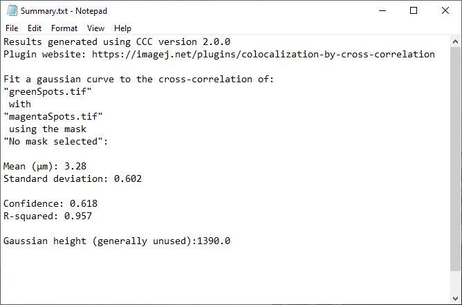 Gaussian fit result
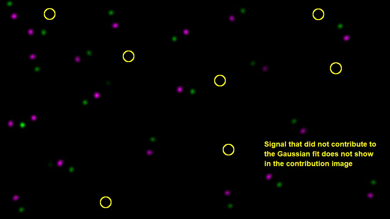 Composit image of Gaussian fit contributions
Here’s a detailed description of each of the result windows:
Correlogram plot
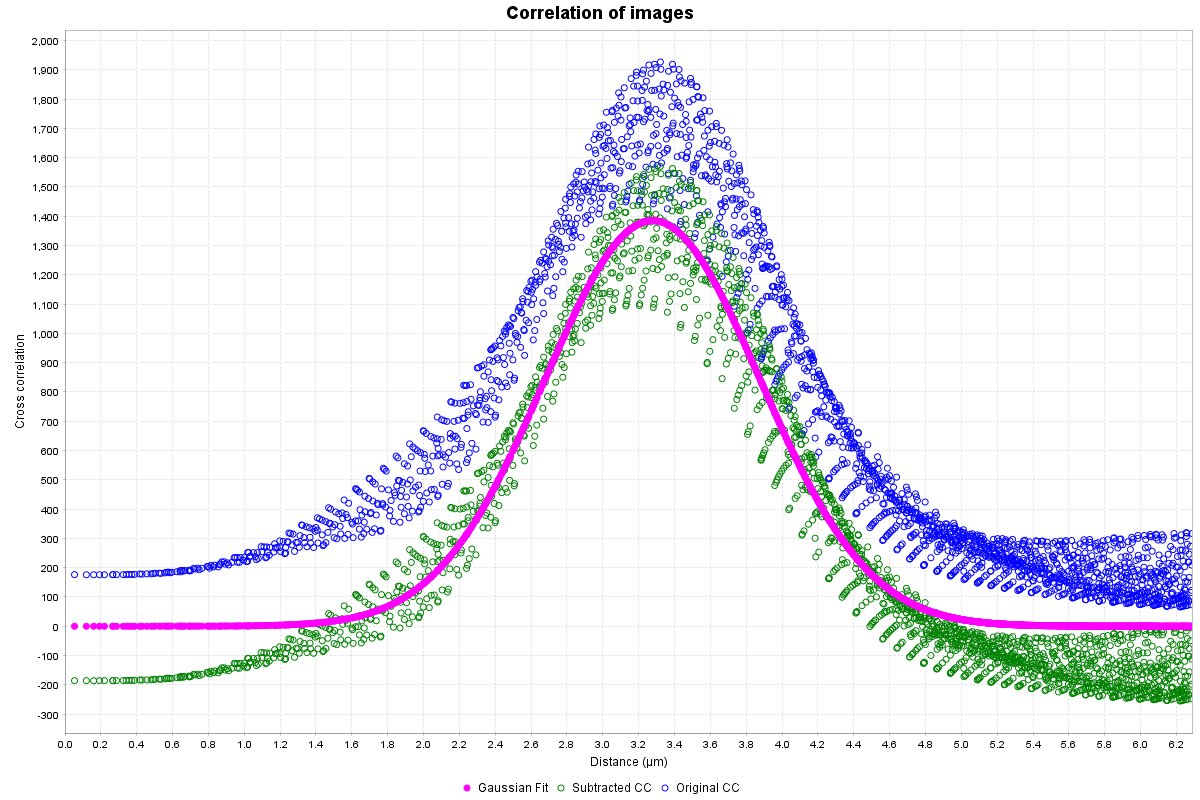
A radial profile plot will be displayed, it contains the radial profile of the original cross-correlation image (blue circles), the radial profile of the cross-correlation after subtraction of low spatial frequency component (green circles), and a Gaussian curve fit to the subtracted profile (magenta filled circles). The distance between the blue and the magenta is a visual indicator of the confidence value described below. The Y-axis is the average of the cross-correlation function. While not technically arbitrary, it is most easily viewed as a measure of relative cross-correlation. The range of the graph is set automatically to fit the Gaussian curve. If you wish to view all the data right click the plot and select Auto Range > Both Axes.
Gaussian fit analysis
This table will contain (in scaled units), the mean distance for the measured correlation (µ), the standard deviation of that correlation (σ), and the peak height of the Gaussian fit. It also contains the statistical measures confidence and R-squared. Each parameter is explained below in detail, including limitations and methods to improve on that parameter.
Mean/µ
Simply the average distance of the measured spatial correlation from the Gaussian curve fitting. The Gaussian fit function has never returned an exact zero value, so make sure to round extremely small values (e.g. 1.2E-17) to zero. Additionally, be careful interpreting these zero values, or any value below the resolution limit. In many other colocalization methods, only spatial correlations within this range would result in positive “colocalization”. With CCC, values of or near zero generally mean that the resolution of the image was too low to determine the true average spatial correlation distance, but that it is likely somewhere in the range of 0 to σ or 2σ. You could get a more precise measure of the correlation distance with improved resolution, though this may not be necessary for your research. That being said, from testing so far (and because of how CCC works), it does seem that CCC can return accurate mean values a little below the resolution limit in some rare cases. This can occur because we are aggregating all the correlating particles within the image. However, to be interpreted as such, the results should be consistent across experimental repeats. It’s much more likely to be a fluke than super-resolved results.
Standard Deviation/σ
The standard deviation of the measured spatial correlation. Generally speaking, this value can be improved by improving the input image resolution. However, the returned value could also be caused by true variability in the measured spatial correlation. Abnormally high values (e.g. σ values of ~7-10µm for an image of a single cell) are usually caused by an inappropriate mask or complete lack of mask when one is justified, or by the resolution being too low for the high molecular density in one or both of the images.
Confidence
Confidence is a novel metric specific to CCC. It is determined by taking the area under the curve (AUC) of the Gaussian fit curve (in range of mean ± 3×sigma) divided by the AUC of the original correlation radial profile (in same range). Values closer to 1 indicate a strong likelihood of true correlation. Values near 0 indicate low to no correlation between the two images, or that more resolution is needed. I currently estimate that values of ~0.10 or greater indicate a reasonably likley correlation (within the range specified by the Gaussian curve), with values of 0.2 or greater indicating a likely true correlation. Ultimately, it is more important to have consistent results across experimetal repeats than a confidence above 0.2.
The confidence is influenced by many image quality and spatial correlation parameters, including image resolution, molecular density, correlation distance, non-correlated particles, and image background. Generally speaking, low confidence values can be increased by improving image resolution. However, this assumes a true spatial correlation exists, as low confidence can also simply indicate a lack of a true correlation. If your confidence is very low, make sure you are pre-processing your images correctly and subtracting image background on a 32-bit image.
R-squared
The R-squared value is also only calculated in the range of mean ± 3×sigma, and is mostly affected by the noise in the image, and the degree of anisotropy of the PSF. Generally speaking, assuming the signal to noise ratio is reasonable, R-squared is not going to be something to worry about.
Gaussian peak height
The peak height can likely be ignored in most cases, but loosely reflects the relative strength of the correlation. As an example, it could be used if you expect a change in the number of correlated particles or ratio of correlated to uncorrelated particles, but no change in the distance. Since the Gaussian curve fitting is done off the subtracted cross-correlation data, the peak height is also influenced by all the image quality parameters that confidence is. For the height to be comparable across images, they must have been imaged under identical conditions. Importantly, the values in the cross-correlation results are normalized to the mask volume. Thus, differences in the volume of anlayzed region should be accounted for if you are comparing Gaussian height.
Contribution of each image to the Gaussian fit
Two new images will be created that display the signal from each analyzed image that contributed to the cross-correlation and Gaussian fit result. It is important to note that the data it contains will always be visible, even if you do NOT have a strong correlation between the two images. Generally, the pixel intensity values should NOT be used as an indicator of overall correlation between the images, but the relative brightness within an image can be used as an approximate indicator of how strongly that particular signal contributed to the correlation result. This relative brightness indication can be easily seen in the example data above: In our original data, all the dots are of the same size and intensity, however, in the resulting contribution images, the dots that remain are varied in their brightness based on how much they contributed to the cross-correlation result (you’ll notice that the brightest dots are all oriented in the same direction).
Multi-Gaussian curve fitting
As of v2.3.0, CCC now natively supports the fitting of multiple Gaussians to data as a sum-of-Gaussians curve. The number of Gaussian terms to attempt to fit is set at the dialog pop-up when running CCC. Mutli-term Gaussian curves can be useful if the spatial relation between your two images has multiple components, most often a broad low-frequency component and a narrow high-frequency component with similar mean values. The confidence value is calculated independently for each Gaussian term, thus over-fitting can result in reducing the confidence of each individual Gaussian term. Also, every additional Gaussian term in the fitting process adds additional computation time.
Working with time-series data:
Working with time-series data is not that different than working with non-time-series data. Every frame of your data is analyzed individually, in the exact same manner that non-time-series data would be analyzed. Thus, all inputs (including the mask) must have the same number of frames. The output generated from the plugin has been changed to better suit time-series data:
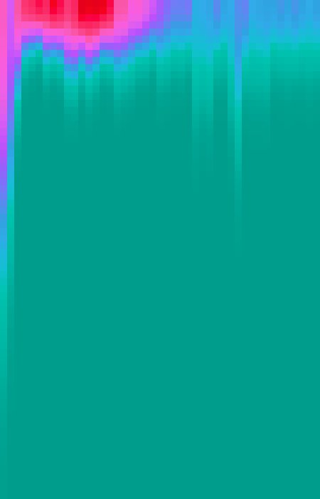
Heat map of Gaussian fit: An example of the heat map generated with time-series data, shown with the Ice lookup table. Each column of pixels shows the Gaussian curve fit to the cross-correlation for a single frame.
The most noteable difference with time-series data is how the data for the correlation plot is displayed. Instead of scatter-graphs, the plugin generates heat maps, where the x-axis is time, the y-axis is distance with 0 at the top, and the intensity is the average of the cross-correlation function at that distance. As we cannot simultaneously show the data for the three lines that would be shown in the correlation plot when using a heat map, we instead generate a three channel image. The first channel (defaults to magenta), displays the Gaussian curve fit to the profile of correlation after subtraction of random associations, equivalent to the magenta circles from the correlation plot. The second channel (defaults to green) shows the cross-correlation function results after subtraction of random associations, equivalent to the green circles from the correlation plot. And the third channel (defaults to blue) show the results of the original cross-correlation function, equivalent to the blue circle from the correlation plot.
Another change with time-series data is that in addition to the Gaussian fit analysis text window, which now displays the fit data for the frame with the highest correlation, the plugin will output a table of Gaussian fit results, showing the Gaussian fits and confidence for each frame. To save this table (if you didn’t use the auto-save feature), go to File > Export > Table…, click browse and save the file as a .csv file (you must add the extension or you will get an error message).
Lastly, the contribution images will still be generated and are functionally the same as for their non-time series counterparts. However, it’s important to note that the contribution is evaluted on a per frame basis, and thus each frame shows the signal contribution to the Gaussian fit results for that frame. Thus, if your cross-correlation distance shifts over the course of an experiment, the contribution images will display this shifting correlation.
Advantages and Disadvantages
Advantages
- High- and super-resolution compatible: Since CCC measures spatial correlation over as a function of distance, there’s no requirement for the two channels to overlap. This means that you can keep improving your resolution, and your results will generally just get better (there is a limit to this, but it would mean drastically oversampling your data).
- More details of the spatial correlation are provided, leading to a better understanding of the nature of the relation
- Image quality metrics and spatial correlation variability are built into the results (with zero effort from the user):
- Improved resolution > more accurate mean, narrower SD, higher confidence
- Higher SNR > higher R-squared
- Higher molecular density > lower confidence
- Longer spatial correlation distance > lower confidence, lower R-squared, eventually larger SD; This may seem disadvantageous, but it simply means there’s a slight bias for closer correlations, which are generally more likely to be the true correlation
- More uncorrelated particles > lower confidence, eventually causes inaccuarte mean, larger SD, and lower R-squared
Disadvantages
- The pre-processing steps are important: failure to subtract background will result in low confidence, and failure to use a mask when necessary will often result in fitting to a low spatial frequency (such as cells correlating with themselves and resulting in a mean of 0, and a SD of 5-10 µm)
- Results are sensitive to mask selection: changes to the mask can cause significant changes to the results. If very slight mask changes cause significant changes to the results it likely means you are right on the border of the required resolution for the spatial correlation you are measuring, and you should try to improve your resolution
- The plugin uses a lot of memory, more than I ever thought it would, and nearly all the memory used scales with image size. I’ve tried reducing the memory requirement as much as I can, but it still uses a ton. Changing the input image bit-depth makes almost no difference, as all the calculations and data generated are 32-bit. However, there are some things you can do:
- Crop or split the image. If you’re studying correlations inside a cell, you could analyze each cell individually. I don’t recommend cutting across a mask though, this will change your results.
- Turn off intermediate images and contribution images. Both of these add a significant amount to the total memory required for the plugin.
- Buy more RAM. It’s not that expensive, and it’s usually super easy to install. This may not be an option if you use a Mac though.
- Run the analysis with a cloud computing service. CCC was made using SciJava and is Headless mode compatible, making it possible to run the analysis remotely.
How it works & intermediate images description:
First, this plugin applies the provided mask to both images, setting any pixels outside the masked region to zero. If this were not done, these pixels would contribute to the original cross-correlation result, but this contribution would then always subtracted out during the process described below, leading to a decrease in confidence. After applying the mask, this plugin then performs an initial cross-correlation to create a original cross-correlation image. Bright regions in the cross-correlation image correspond to a high correlation between the images when the second image is shifted by a vector equal to the distance form the center of the cross-correlation image to the bright region. Thus, if you see a bright spot in the cross-correlation image that is 2 µm to the left of the image center, it means their is a positive correlation between image 1 and image2 when image2 is shited left 2 µm.
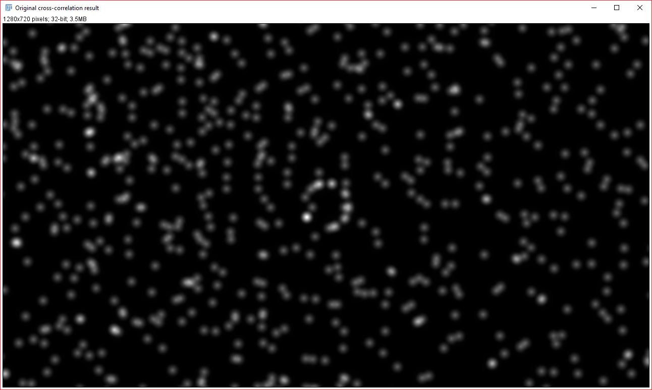 Initial, unmodified cross-correlation result
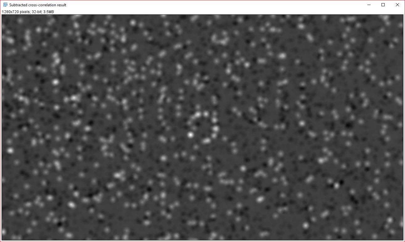 Cross-correlation result after subtraction of low frequency component
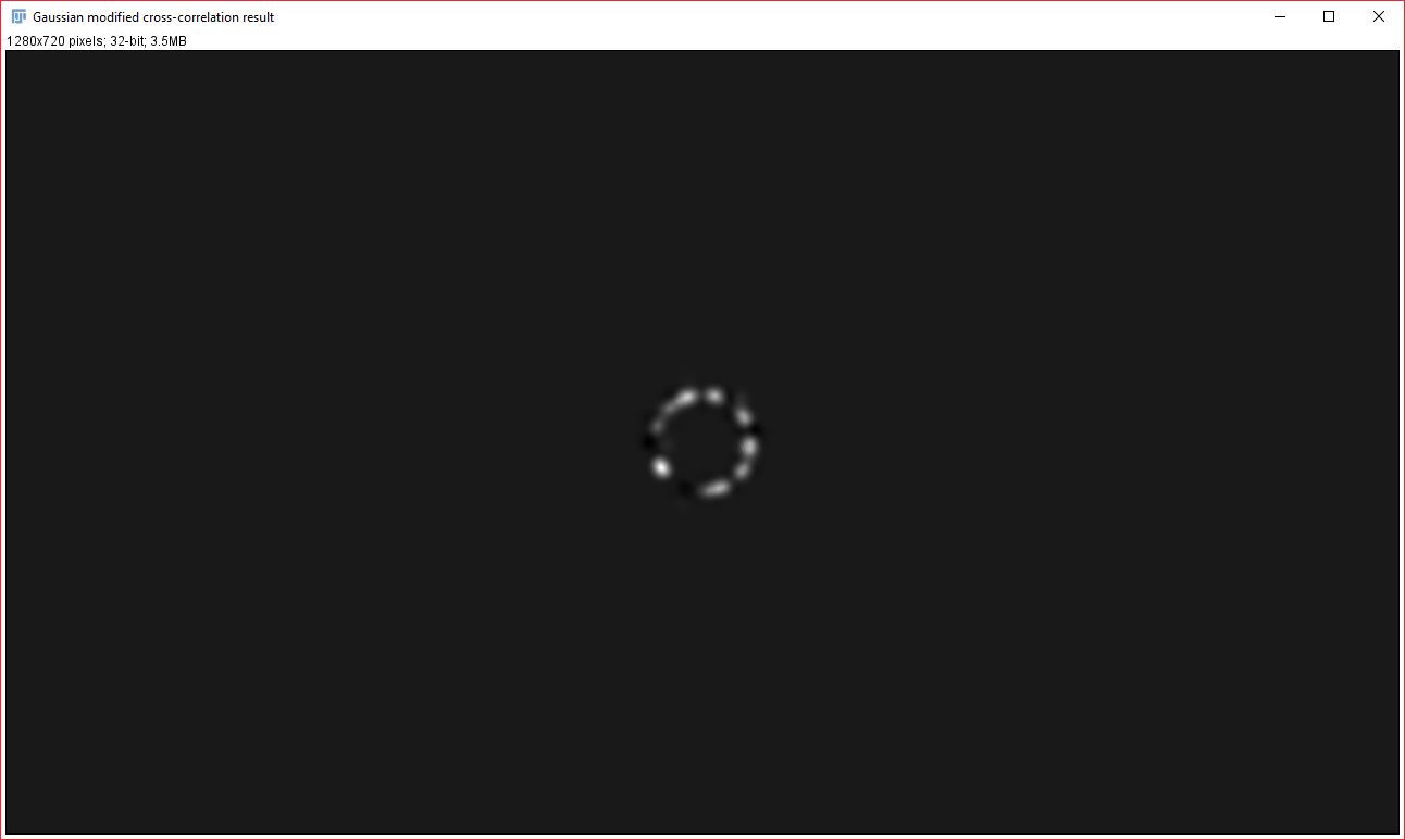 Gaussian-fit modified cross-correlation
To remove the contribution from low spatial frequency structures/data (such as cells and nuclei), a second cross-correlation image generated from a low spatial frequency image is then subtracted from the original correlation image. For this process, the mean intesity of all the pixels of the first input image within the mask is calculated, then a new image is created where all the pixels within the mask are set to this mean value. This image is an averaged low spatial frequency image of your first input image. This low-frequency image is then cross-correlated with the second input image, and the resulting cross-correlation image is the low-frequency component, which is subtracted from the original cross-correlation image. The mean under the mask process is only applied to one image as applying it to both did not result in a significant difference in results and uses more time and memory. Then, we generate a radial profile of the subtracted data and fit a Gaussian curve to it. We also generate a radial profile for the original correlation data before subtraction, as this is needed to establish a measure of confidence. The confidence is calculated as the area under the curve (AUC) of the subtracted correlation radial profile (in the range of mean ± 3×sigma) divided by the AUC of the original correlation radial profile (in same range). The confidence value, along with the mean and sigma of the Gaussian fit are displayed in a log window. Higher values of confidence, closer to 1, indicate that two images likely have a true spatial correlation at the indicated distance.
To generate the contribution images, we further modify the subtracted cross-correlation image, by effectively multiplying it with the Gaussian fit in order to create a cross-correlation image that only retains the data within our Gaussian curve range. This Gaussian-modified cross-correlation image is then used to back-calculate the contribution images. Image1Contribution = (image2 ∗ gaussModifiedCorr) × image1. Image2Contribution = (image1 ★ gaussModifiedCorr) × image2. Key: ∗ -> convolve, ★ -> correlate.
Alternate commands
These commands can be found with CCC under Analyze > Colocalization > Colocalization by Cross Correlation. Use of these is recommended only if the original CCC fails due to lack of memory (and no higher memory computer is available), or if you are generating the cross-correlation data for a purpose other than colocalization.
CCC - No confidence
The no confidence command of CCC is very similar to the original command described above, but it does not calculate the original cross-correlation. Instead, it is able to remove the low-frequency contribution prior to the first cross-correlation and generate the subtracted cross-correlation result without ever generating the original. The downside of this is that it is now unable to calculate the confidence value, as this requires the original cross-correlation data. The no confidence version is not meant for data that generates low confidence results. This is meant solely for very large datasets that are unable to be processed by the original CCC due to memory constraints. Even in these instances, the best practice would be to take a cropped region of the original dataset and perform CCC to get an approximation of the confidence value for the dataset.
As a note: for time-lapse data, since the “best” frame cannot be evaluted using confidence, the frame with the smallest standard deviation is used instead. For this reason, the best frame can differ dramatically between the original version and the no-confidence version of CCC.
Just Cross-correlation
The “Just Cross Correlation” This command simply cross-correlates the two input images, and calculates the radial profile. No Gaussian curve fitting or statistics are calculated. Just cross-correlation can be used if CCC and CCC - No Confidence fail due to insufficient memory, allowing you to at least see a cross-correlation curve, or it can be used for non-Gaussian relations such as the one desscribed below.
I originally made this as I had someone who wanted to determine the average thickness of a joint from a microCT scan. The cross-correlation of an edges only version of the two bones on either side of the joint generated an S-curve (that trailed down after the peak but too slowly for a Gaussian fit), after which they could extract the curve data and fit an S-curve to it using a separate application.
Major revisions
New results table order in v2.3
The parameter order in the results table has been changed to accomadate multiple Gaussian fitting. This change in order will likely affect script results that automatically read from this output table. Order changed from {Mean, SD, Confidence, R-Squared, Height} to {<Mean, SD, Height, Confidence> (per Gaussian), R-Squared}.
New confidence value calculation in v2.3
With the release of the multi-Gaussian fitting in v2.3, the confidence calculation was changed to use the area under the curve (AUC) of the Gaussian fit curve in place of the subtracted correlogram data. This was changed so that each individual Gaussian of a multi-Gaussian fit would have its own confidence value.
Slightly different results in v2.1
In v2.1 of CCC, the way that the low-frequency component of the data is removed from the cross-correlation was altered to allow creation of the “no confidence” command. Basically, instead of cross-correlating a low-frequency component of image 1 (mask with mean value image) with image 2, as described above in the how it works section, in v2.1 the mean pixel value within the mask is subtracted from every pixel of image 1 that is within the mask bounds before it is cross-correlated with image 2. This effectively subtracts the low-frequency component before the cross-correlation is performed, rather than after. During testing, this process generated either identical or very similar results to the version 2 method that is described above. I believe the reason it was not always identical was due to differences in rounding, since the new v2.1 method skips a couple rounding steps from v2. I made this change for both the No confidence command and the original CCC command as I wanted them to produce identical results, and because this method was more memory efficient.
I am not changing the description for “How it works” above, as I feel that is a little easier to understand and the result is effectively the same.
Removing pixel randomization
In v2 of CCC, the repeating pixel randomization process (as described in the BMC Bioinformatics publication) was replaced by the mean within the mask method to remove the low spatial frequency component. This new process was faster, more memory efficient, and allows CCC to generate consistent results when provided the same input. While it seems very different on its face, this is in effect the same process and produces identical results if infinite repeats were used with v1. This is ultimately because the cross-correlation did not have to be done after each randomization with the overall result being averaged across repeats, but instead the randomization of the image could be repeated and averaged first, then the resulting image cross-correlated with the second image. Effectively:
\[\lim\limits_{n \to \infty} \left(\frac{\sum_{i=1}^n \left(rand(Img1)_i \star Img2\right)}{n}\right) = \lim\limits_{n \to \infty} \left(\left(\frac{\sum_{i=1}^n \left(rand(Img1)_i\right)}{n} \right)\star Img2\right)\]The process of randomizing and averaging an image an infinite number of times would result in an image of just the mean intensity value. Hence why the mean intensity under the mask is used.