The content of this page has not been vetted since shifting away from MediaWiki. If you’d like to help, check out the how to help guide!
Description
The BigDataViewer is a re-slicing browser for terabyte-sized multi-view image sequences. BigDataViewer was developed with multi-view light-sheet microscopy data in mind and integrates well with Fiji’s SPIMage processing pipeline.
Conceptually, the visualized data comprises multiple data sources. Each source provides one 3D image (for each time-point in the case of a time-lapse sequence). For example, in a multi-angle SPIM sequence, each angle is a source. In a multi-angle, multi-channel SPIM sequence, each channel of each angle is a source.
BigDataViewer comes with a custom data format that is is optimized for fast random access to very large data sets. This permits browsing to any location within a multi-terabyte recording in a fraction of a second.
The file format is based on XML and HDF5. Images are represented as tiled multi-resolution pyramids, and stored in HDF5 chunked multi-dimensional arrays. The XML file contains metadata, for example the registration of sources to the global coordinate system.
Installation
The BigDataViewer comes with Fiji. You should have a sub-menu Plugins › BigDataViewer.
Usage
Opening a Dataset
To use the BigDataViewer we need some example dataset to browse. There are various options:
Multi-view data converted to XML/HDF5
A special purpose of BigDataViewer is to visualise multi-view light sheet microscopy datasets. Our custom XML/HDF5 is a special purpose hierarchical data format that optimises access to any part of large-multi view datasets using ImgLib2. You can download a small dataset from here, comprising two views and three time-points. This is an excerpt of a 6 angle 715 time-point sequence of drosophila melanogaster embryonal development, imaged with a Zeiss Lightsheet Z.1. Download both the XML and the HDF5 file and place them somewhere next to each other.
Alternatively, you can create a dataset by exporting your own data as described below.
To start BigDataViewer, select Plugins › BigDataViewer › Open XML/HDF5 from the Fiji menu. This brings up a file open dialog. Open the XML file of your test dataset.
Standard microscopy data
The BigDataViewer can be used to visualise and navigate any image that can be opened in Fiji. Since Fiji relies of LOCI Bioformats library that means essentially all know microscopy file formats.
For example, open the sample image File › Open Samples › Mitosis (26MB, 5D stack) from the Fiji menu. Subsequently select Plugins › BigDataViewer › Open Current Image which will launch the BigDataViewer with the sample image, for navigation by arbitrary re-slicing.
Imaris files
Imaris (Bitplane) uses a hierarchical data format (similar to BigDataViewer’s XML/HDF5 format). In order to open Imaris .ims files select Plugins › BigDataViewer › Open Imaris (experimental) from the Fiji menu. Please note, that support for the Imaris format is still experimental.
Basic Navigation
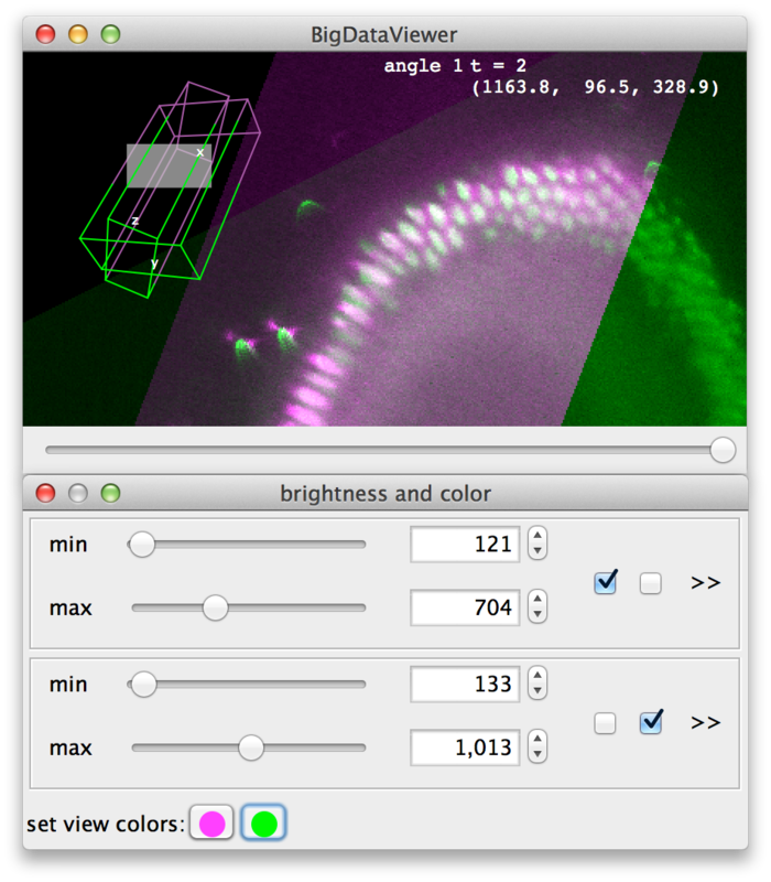
Assuming you downloaded the drosophila melanogaster example dataset, you should see something like this:
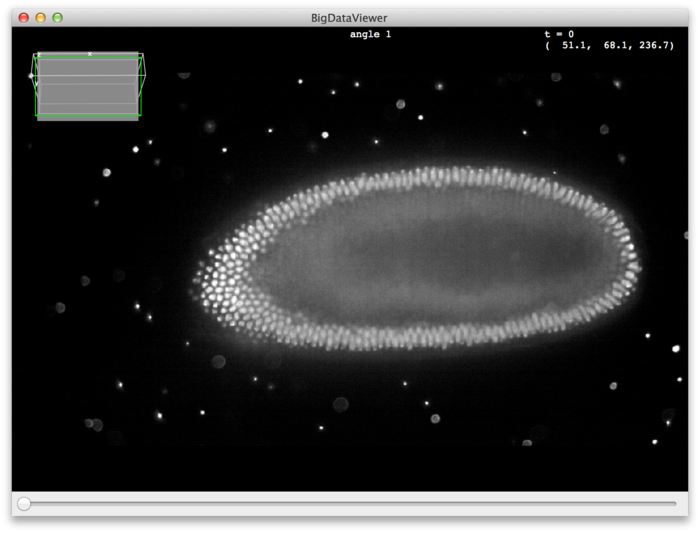
On startup, the middle slice of the first source (angle) is shown. You can browse the stack using the keyboard or the mouse. To get started, try the following:
- Use the mouse-wheel or < and > keys to scroll through z slices.
 Right Drag anywhere on the canvas to translate the image.
- Use ⌃ Ctrl + ⇧ Shift +
 Mouse Wheel, or ↑ Up and ↓ Down keys to zoom in and out.
  Left Drag anywhere on the canvas to rotate (reslice) the image.
The following table shows the available navigation commands using the mouse:
|
|
Rotate (pan and tilt) around the point where the mouse was clicked. |
|
|
Translate in the XY-plane. |
|
|
Move along the z-axis. |
|
⌘ Command + |
Zoom in and out. |
The following table shows the available navigation commands using keyboard shortcuts:
|
X, Y, Z |
Select keyboard rotation axis. |
|
← Left, → Right |
Rotate clockwise or counter-clockwise around the choosen rotation axis. |
|
↑ Up, ↓ Down |
Zoom in or out. |
|
,, . |
Move forward or backward along the Z-axis. |
|
⇧ Shift + X |
Rotate to the ZY-plane of the current source. (Look along the X-axis of the current source.) |
|
⇧ Shift + Y or ⇧ Shift + A |
Rotate to the XZ-plane of the current source. (Look along the Y-axis of the current source.) |
|
⇧ Shift + Z |
Rotate to the XY-plane of the current source. (Look along the Z-axis of the current source.) |
|
[ or N |
Move to previous timepoint. |
|
] or M |
Move to next timepoint. |
For all navigation commands you can hold ⇧ Shift to rotate and browse 10x faster, or hold ⌃ Ctrl to rotate and browse 10x slower. For example, ← Left rotates by 1° clockwise, while ⇧ Shift + ← Left rotates by 10°, and ⌃ Ctrl + ← Left rotates by 0.1°.
The axis-rotation commands (e.g., ⇧ Shift + X) rotate around the current mouse location. That is, if you press ⇧ Shift + X, the view will pivot such that you see a ZY-slice through the dataset (you look along the X-axis). The point under the mouse will stay fixed, i.e., the view will be a ZY-slice through that point.
Interpolation Mode
Using I you can switch between nearest-neighbor and trilinear interpolation schemes. The difference is clearly visible when you zoom in such that individual source pixels are visible.
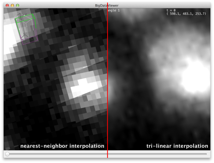
Trilinear interpolation results in smoother images but is a bit more expensive computationally. Nearest-neighbor is faster but looks more pixelated.
Displaying Multiple Sources
BigDataViewer datasets typically contain more than one source. For a SPIM sequence one usually has multiple angles and possibly fused and deconvoled data on top.
Select Settings › Visibility & Grouping from the BigDataViewer menu to bring up a dialog to control source visibility. You can also bring up this dialog by the shortcut F6.
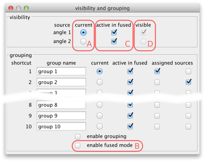
Using the current source checkboxes (A in the figure above), you can switch between available sources. The first ten sources can also be made current by the number keys 1 through 0 in the main BigDataViewer window.
To view multiple sources overlaid at the same time, switch to fused mode using the checkbox (B). You can also switch between normal and fused mode using the shortcut F in the main window. In fused mode individual sources can be turned on and off using the checkboxes (C) or shortcuts ⇧ Shift + 1 through ⇧ Shift + 0 in the main window.
Whether in normal or fused mode, the (unselectable) boxes (D) provide feedback on which sources are actually currently displayed. Also the main window provides feedback:
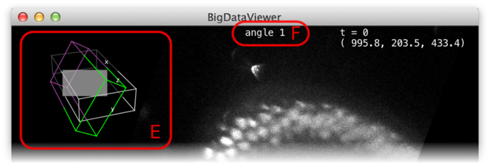
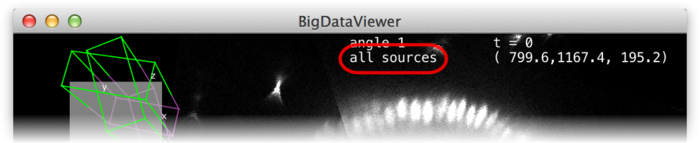
In the top-left corner an overview of the dataset is displayed (E). Visible sources are displayed as green/magenta wireframe boxes, invisible sources are displayed as grey wireframe boxes. The dimensions of the boxes illustrate the size of the source images. The filled grey rectangle illustrates the screen area, i.e., the portion of the currently displayed slice. For the visible sources, the part that is in front of the screen is green, the part that is behind the screen is magenta.
At the top of the window, the name of the current source is shown (F).
Note, that also in fused mode there is always a current source, although this source may not even be visible. Commands such as ⇧ Shift + X (rotate to ZY-plane) refer to the local coordinate system of the current source.
Grouping Sources
Often there are sets of sources for which visibility is logically related. For example, in a multi-angle, multi-channel SPIM sequence, you will frequently want to see all channels of a given angle, or all angles of a given channel. If your dataset contains deconvolved data, you may want to see either all raw angles overlaid, or the deconvolved view, respectively. You want to be able to quickly switch between those two views. Turning individual sources on and off becomes tedious in these situations. Therefore, sources can be organized into groups. All sources of a group can be activated or deactivated at once.
Source grouping is handled in the visibility and grouping dialog, too (menu Settings › Visibility & Grouping or shortcut F6).
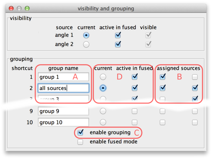
The lower half of the dialog is dedicated to grouping. There are 10 groups available. They are named “group 1” through “group 10” initially, but the names can be edited (A).
Sources can be assigned to groups using the checkboxes (B). In every line, there are as many checkboxes as there are sources. Sources corresponding to active checkboxes are assigned to the respective group. For example, in the above screenshot there are two sources and therefore two “assigned sources” checkboxes per line The first source is assigned to groups 1 and 2, the second source is assigned to groups 2 and 3. Group 2 has been renamed to “all sources”.
Grouping can be turned on and off by the checkbox (C) or by using the shortcut G in the main window. If grouping is enabled, groups take the role of individual sources: There is one current group which is visible in normal mode (all individual sources that are part of this group are overlaid). Groups can be activated or deactivated to determine visibility in fused mode (all individual sources that are part of at least one active group are overlaid).
Groups can be made current and made active or inactive using the checkboxes (D). Also, if grouping is enabled the number key shortcuts in the main BigDataViewer window act on groups instead of individual sources. That is, groups 1 through 10 can be made current by keys 1 through 0. Similarly, shortcuts ⇧ Shift + 1 through ⇧ Shift + 0 in the main window activate or deactivate groups 1 through 10 for visibility in fused mode.
If grouping is enabled, the name of the current group is shown at the top of the main window.
Adjusting Brightness and Color
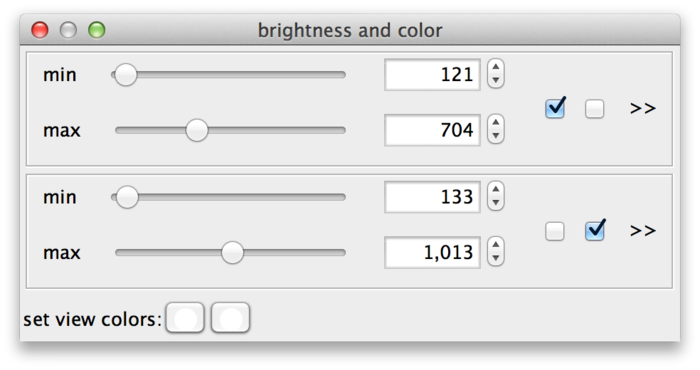
To change the brightness, contrast, or color of particular sources select Settings › Brightness & Color or press the shortcut S. This brings up the brightness and color settings dialog.
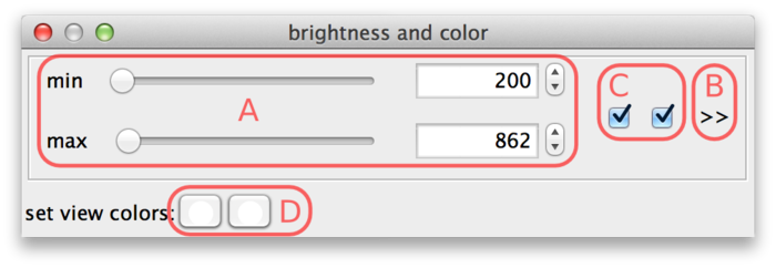
The min and max sliders (A) can be used to adjust the brightness and contrast. They represent minimum and maximum source values that are mapped to the display range. For the screenshot above, this means that source intensity 200 (and everything below) is mapped to black. Source intensity 862 (and everything above) is mapped to white.
When a new dataset is opened, BigDataViewer tries to estimate good initial min and max settings by looking at the first image of the dataset.
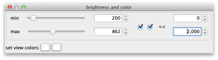
BigDataViewer datasets are currently always stored with 16 bits per pixel, however the data does not always exploit the full value range 0 … 65535. The example drosophila dataset uses values in the range of perhaps 0 … 1000, except for the much brighter fiducial beads around the specimen. The min and max sliders in this case are a bit fiddly to use, because they span the full 16 bit range with the interesting region squeezed into the first few pixels. This can be remedied by adjusting the range of the sliders. For this, click on the >> dialog button (B). This shows two additional input fields, where the range of the sliders can be adjusted. In the following screenshot, the leftmost value of the slider range has been set to 0 and the rightmost value to 2000, making the sliders much more useful.
So far, all sources share the same min and max settings. However, these can also be adjusted for each individual source or for groups of sources. The checkboxes (C) assign sources to min-max-groups. There is one checkbox per source. In the example drosophila dataset there are two sources, therefore there are two checkboxes. The active checkboxes indicate for which sources the min and max values apply.
If you uncheck one of the sources, it will move to its own new min-max-group. Now you can adjust the values for each source individually. The sliders of new group are initialized as a copy of the old group.
Sources can be assigned to min-max-groups by checking/unchecking the checkboxes. The rule is that every source is always assigned to exactly one min-max-group. Thus, if you activate an unchecked source in a min-max-group, this will remove the source from its previous min-max-group and add it to the new one. Unchecking a source will remove it from its min-max-group and move it to a new one. Min-max-groups that become empty are removed. To go back to a single min-max-group in the example, you would simply move all sources to the same group.
Finally, at the bottom of the dialog (D) colors can be assigned to sources. There is one color button per source (two in the example). Clicking a button brings up a color dialog, where you can choose a color for that particular source. In the following screenshot, the sources have been colored magenta and green.
Bookmarking Locations and Orientations
BigDataViewer allows to bookmark the current view. You can set bookmarks for interesting views or particular details of your dataset to easily navigate back to those views later.
Each bookmark has an assigned shortcut key, i.e., you can have bookmarks “a”, “A”, “b”, …, “1”, “2”, etc. To set a bookmark for the current view, press ⇧ Shift + B and then the shortcut you want to use for the bookmark. To recall bookmark, press B and then the shortcut of the bookmark.
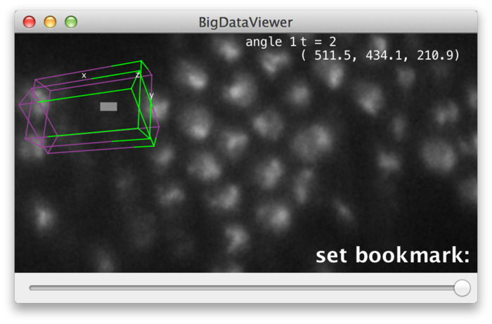
BigDataViewer provides visual feedback for setting and recalling bookmarks. When you press ⇧ Shift + B, the message “set bookmark:” appears in the lower right corner of the main window, prompting to press the bookmark shortcut next.
Now press the key you want to use as a shortcut, for example A. The prompt message will change to “set bookmark: a” indicating that you have set a bookmark with shortcut A. Instead of pressing a shortcut key you can abort using ⎋ Esc.
Similarly, when you press B to recall a bookmark, the prompt message “go to bookmark:” appears. Now press the shortcut of the bookmark you want to recall, for example A. The prompt message will change to “go to bookmark: a” and the view will move to the bookmarked location. Instead of pressing a shortcut key you can abort using ⎋ Esc.
Note, that bookmark shortcuts are case-sensitive, i.e., A and ⇧ Shift + A refer to distinct bookmarks “a” and “A” respectively.
The bookmarking mechanism can also be used to bookmark and recall orientations. Press O and then a bookmark shortcut to recall only the orientation of that bookmark. This rotates the view into the rotation of the bookmarked view (but does not zoom or translate to the bookmarked location). The rotation is around the current mouse location (i.e., the point under the mouse stays fixed).
Loading and Saving Settings
Organizing sources into groups, assigning appropriate colors, adjusting brightness correctly, and bookmarking interesting locations is work that you do not want to repeat over and over every time you re-open a dataset. Therefore, BigDataViewer allows to save and load these settings.
Select File › Save settings from the menu to store settings to an XML file, and File › Load settings to load them from an XML file.
When a dataset is opened, BigDataViewer automatically loads an appropriately named settings file if it is present. This settings file must be in the same directory as the dataset’s XML file, and have the same filename with .settings appended. For example, if the dataset’s XML file is named drosophila.xml, the settings file must be named drosophila.settings.xml. (If you select File › Save settings, this filename is already suggested in the Save File dialog.)
Settings files assume that a specific number of sources are present, therefore settings are usually not compatible across different datasets.
Opening BigDataViewer Datasets as ImageJ Stacks
BigDataViewer may be great for looking at your data, but what if you want to apply other ImageJ algorithms or plugins to the images? You can open individual images from a dataset as ImageJ stacks using File › Import › BigDataViewer… from the Fiji menu.
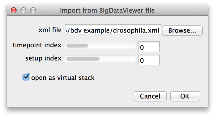
Select the XML file of a dataset, then choose the time-point and source (setup) index of the image you want to open. If you enable the “open as virtual stack” checkbox the image will open as an ImageJ virtual stack. This means that the opened image is backed by BigDataViewer’s cache and slices are loaded on demand. Without “open as virtual stack”, the full image will be loaded into memory. Virtual stacks will open a bit faster but switching between slices may be less instantaneous.
Note that the import function is macro-recordable. Thus, you can make use of it to batch-process images from BigDataViewer datasets.
Exporting Datasets for the BigDataViewer
BigDataViewer uses a custom file-format that is optimized for fast arbitrary re-slicing at various scales. This file format is build on open standards XML and HDF5. XML is used to store meta-data and HDF5 is used to store image volumes. (Actually, we support several ways to store the image volumes besides HDF5. For example, the volume data can be provided by a web service for remote access.)
Before we discuss how to export your data to this XML/HDF5 format, we provide a rough overview for some background, rationale, and terminology. The format is explained in detail in our paper BigDataViewer: Interactive Visualization and Image Processing for Terabyte Data Sets.
About the BigDataViewer data format
Each BigDataViewer dataset contains a set of 3D grayscale image volumes organized by timepoints and setups. In the context of lightsheet microscopy, each channel or acquisition angle or combination of both is a setup. E.g., for a multi-view recording with 3 angles and 2 channels there are 6 setups. Each setup represents a visualisation data source in the viewer that provides one image volume per timepoint. We refer to each combination of setup and timepoint as a view. Each view has one corresponding grayscale image volume.
A dataset comprises an XML file to store meta-data and one or more HDF5 files to store the raw images. Among other things, the XML file contains
- the path of the HDF5 file(s),
- a number of setups,
- a number of timepoints,
- the registration of each view into the global coordinate system.
Each view has one corresponding image volume which is stored in the HDF5 file. Raw image volumes are stored as multi-resolution pyramids: In addition to the original resolution, several progressively down-scaled resolutions (mipmaps) are stored. This serves two purposes. First, using mipmaps minimizes aliasing effects when rendering a zoomed-out view of the dataset~\cite{Williams:1983it}. Second, and more importantly, using mipmaps reduces data access time and thus increases the perceived responsiveness for navigation. Low-resolution mipmaps take up less memory and therefore load faster from disk. New chunks of data must be loaded when the user browses to a part of the dataset that is not currently cached in memory. In this situation, BigDataViewer can rapidly load and render low-resolution data, filling in high resolution detail later as it becomes available. This multi-resolution pyramid scheme is illustrated in the following figure.
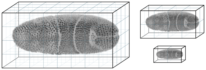
Each raw image volume is stored in multiple resolutions, the original resolution (left) and successively smaller, downsampled versions (right). Each resolution is stored in a chunked representation, split into small 3D blocks.
Each level of the multi-resolution pyramid is stored as a chunked multi-dimensional array. Multi-dimensional arrays are the standard way of storing image data in HDF5. The layout of multi-dimensional arrays on disk can be configured. We use a chunked layout which means that the 3D image volume is split into several chunks (smaller 3D blocks). These chunks are stored individually in the HDF5 file, which optimizes performance for our use-case where fast random access to individual chunks is required.
Rendering a virtual slice requires data contained within a small subset of chunks. Only chunks that touch the slice need to be loaded, as illustrated in the following Figure.
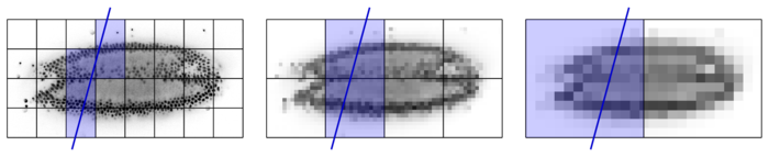
When rendering a slice (schematically illustrated by the blue line) the data of only a small subset of blocks is required. In the original resolution 5 blocks are required, while only 2, respectively 1 block is required for lower resolutions. Therefore, less data needs to be loaded to render a low-resolution slice. This allows low-resolution versions to be loaded and rendered rapidly. High-resolution detail is filled in when the user stops browsing to view a certain slice for an extended period of time.
Each of these chunks, however, is loaded in full, although only a subset of voxels in each chunk is required to render the actual slice. Loading the data in this way, aligned at chunk boundaries, gurantees optimal I/O performance.
All loaded chunks are cached in RAM. During interactive navigation, subsequent slices typically intersect with a similar set of chunks because their pose has changed only moderately, i.e.. cached data are re-used. Only chunks that are not currently in the cache need to be loaded from disk, as illustrated in the following Figure.
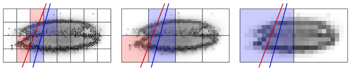
For rendering the slice indicated by the red line, only the red blocks need to be loaded. The blue blocks are already cached from rendering the blue slice before. Combined with the multi-resolution mipmap representation, this chunking and caching scheme allows for fluid interactive browsing of very large datasets.
The parameters of the mipmap and chunking scheme are specific to each dataset and they are fully configurable by the user. In particular, when exporting images to the BigDataViewer format, the following parameters are adjustable:
- the number of mipmap levels,
- the subsampling factors in each dimension for each mipmap level,
- the chunk sizes in each dimension for each mipmap level.
BigDataViewer suggests sensible parameter settings, however, for particular applications and data properties a user may tweak these parameters for optimal performance.
Exporting from ImageJ Stacks
You can export any dataset to BigDataViewer format by opening it as a stack in Fiji and then selecting Plugins › BigDataViewer › Export Current Image as XML/HDF5 from the Fiji menu. If the image has multiple channels, each channel will become one setup in the exported dataset. If the image has multiple frames, each frame will become one timepoint in the exported dataset. Of course, you may export from virtual stacks if your data is too big to fit into memory.
To get started, let’s open one of the ImageJ sample images by File › Open Samples › T1 Head (2.4M, 16-bits). Selecting Plugins › BigDataViewer › Export Current Image as XML/HDF5 brings up the following dialog.
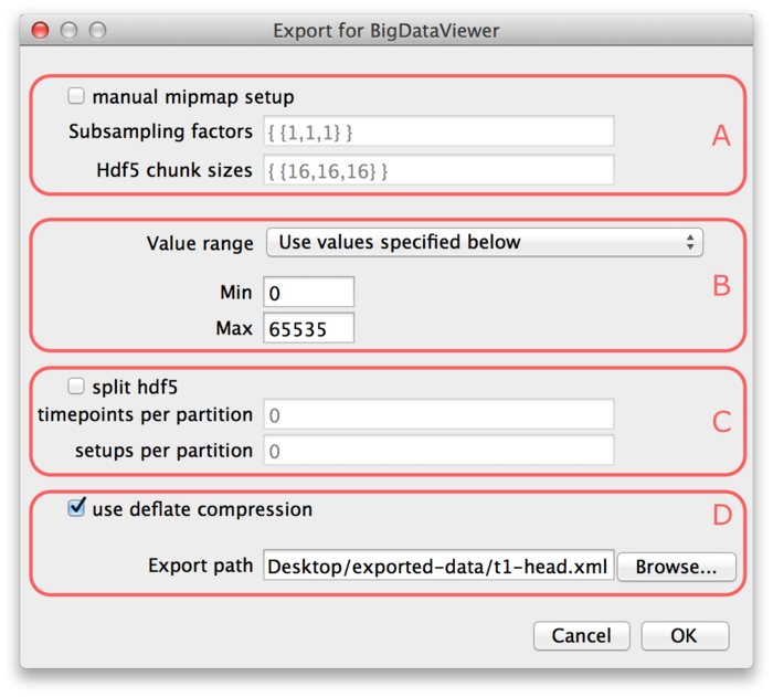
Parts (A) and (C) of the dialog are optional, so we will explain (B) and (D) first.
At the bottom of the dialog (D), the export path is defined. Specify the path of the XML file to which you want to export the dataset. The HDF5 file for the dataset will be placed into the same directory under the same name with extension “.h5”. If the “use deflate compression” checkbox is enabled, the image data will be compressed using HDF5 built-in DEFLATE compression. We recommend to use this option. It will usually reduce the file size to about 50% with respect to uncompressed image size. The performance impact of decompression when browsing the dataset is negligible.
In part (B) of the dialog the value range of the image must be specified. BigDataViewer always stores images with 16-bit precision currently, while the image you want to export is not necessarily 16-bit. The value range defines the minimum and maximum of the image you want to export. This is mapped to the 16-bit range for export. I.e., the minimum of the value range will be mapped to the minimum of the unsigned 16-bit range (0). The maximum of the value range will be mapped to the maximum of the unsigned 16-bit range (65535). In the drop-down menu you can select one the following options to specify how the value range should be determined:
- “Use ImageJ’s current min/max setting”. The minimum and maximum set in ImageJ’s Brightness&Contrast are used. Note, that image intensities outside that range will be clipped to the minimum or maximum, respectively.
- “Compute min/max of the (hyper-)stack”. Compute the minimum and maximum of the stack and use these. Note, that this may take some time to compute because it requires to look at all pixels of the stack you want to export.
- “Use values specified below”. Use the values specified in the Min and Max fields (B) of the export dialog. Note, that image intensities outside that range will be clipped to the minimum or maximum, respectively.
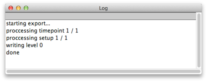
After you have specified the value range and selected and export path, press OK to export the dataset. Messages about the progress of the operation are displayed in the ImageJ Log window.
When the export is done you can browse the dataset in the BigDataViewer by opening the exported XML file.
The optional parts (A) and (C) of the export dialog provide further options to customize the export. If the checkbox “manual mipmap setup” is enabled, you can customize the multi-resolution mipmap pyramid which stores your image stacks. You can specify the number of resolution levels used, and their respective down-scaling factors, as well as the chunk sizes into which each resolution level is subdivided.
The “Subsampling factors” field specifies a comma-separated list of resolution levels, formatted as {level, ..., level}. Each level is a list of subsampling factors in X, Y, Z, formatted as {x-scale, y-scale, z-scale}. For example consider the specification . This will create a resolution pyramid with three levels. The first level is the full resolution – it is scaled by factors 1 in all axes. The second level is down-scaled by factors 2, 2, 1 in X, Y, Z respectively. So it has half the resolution in X and Y, but full resolution in Z. The third level has half the resolution of the second in all axes, i.e., it is down-scaled by factors 4, 4, 2 in X, Y, Z respectively. Note, that you should always order levels by decreasing resolution like this. Also note, that in the above example we down-scale by different factors in different axes. One may want to do this if the resolution of the dataset is anisotropic. Then it is advisable to first downscale only in the higher-resolved axes until approximately isotropic resolution is reached.
The “Hdf5 chunk sizes” specifies the chunk sizes into which data on each resolution level is sub-divided. This is again formatted as {level, ..., level}, with the same number of levels as supplied for the Subsampling factors. Each level is a list of sizes in X, Y, Z, formatted as {x-size, y-size, z-size}. For example consider the specification . This will sub-divide each resolution level into chunks of 16×16×16 pixels.
It is usually not recommended to specify subsampling factors and chunk sizes manually. When browsing a dataset, the mipmap setup determines the loading speed and therefore the perceived speed of browsing to data that is not cached. With “manual mipmap setup” turned off, reasonable values will be determined automatically depending on the resolution and anisotropy of your dataset.
Finally, in part (C) of the export dialog, you may choose to split your dataset into multiple HDF5 files. This is useful in particular for very large datasets. For example when moving the data to a different computer, it may be cumbersome to have it sitting in a single 10TB file. If the checkbox “split hdf5” is enabled the dataset will be split into multiple HDF5 partition files. The dataset can be split along the timepoint and setup dimensions. Specify the number of timepoints per partition and setups per partition in the respective input fields.
For example, assume your dataset has 4 setups and 10 timepoints. Setting timepoints per partition = 5 and setups per partition = 2 will result in 4 HDF5 partitions:
- setups 1 and 2 of timepoints 1 through 5,
- setups 3 and 4 of timepoints 1 through 5,
- setups 1 and 2 of timepoints 6 through 10, and
- setups 3 and 4 of timepoints 6 through 10.
Setting timepoints per partition = 0 or setups per partition = 0 means that the dataset is not split in the respective dimension.
Note, that splitting into multiple HDF5 files is transparent from the viewer side. There is still only one XML file that gathers all the partitions files into one dataset.
Integration with Fiji’s SPIMage Processing Tools
BigDataViewer seamlessly integrates with the “Multiview Reconstruction” plugins that Fiji offers for registration and reconstruction of lightsheet microscopy data. Recent versions of these tools build on the same XML format as BigDataViewer itself. In addition to HDF5, “Multiview reconstruction” supports a backend for datasets that store individual views as TIFF files, because unprocessed data from lightsheet microscopes is often available in this format.
In principle, BigDataViewer is able to display a TIFF dataset as is. However, for quick navigation this is not the ideal format: When navigating to a new timepoint, BigDataViewer needs to load all TIFF files of that timepoint into memory, suffering a delay of tens of seconcds. Therefore, it is beneficial to convert the TIFF dataset to HDF5. Note, that this can be done at any point of the processing pipeline (i.e., before registration, after registration, after multiview fusion or deconvolution, etc) because the “Multiview reconstruction” plugins can operate on HDF5 datasets as well.
We assume that the user has already created an XML/TIFF dataset, as explained in Multiview-Reconstruction.
To convert the dataset to HDF5, select Plugins › Multiview Reconstruction › Resave › As HDF5 form the Fiji menu. This brings up the following dialog.
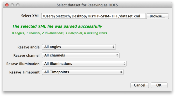
At the top of the dialog, select the XML file of the dataset you want to convert to HDF5. In the lower part of the dialog, you can select which parts of the dataset you want to resave. For example, assume that the source dataset contains the raw image stacks from the microscope, as well as deconvolved versions. You might decide that you do not need the raw data as HDF5, so you can select only the deconvolved channels. Once you have determined what you want to convert press OK.
This brings up the next dialog, in which you need to specify the export path and options.
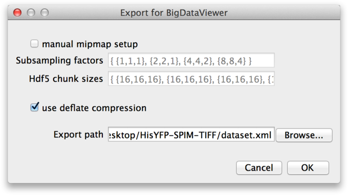
These parameters are the same as discussed in the previous section: If you want to specify custom mipmap settings, you can do so in the top part of the dialog. Below that, choose whether you want to compress the image data. For the export path, specify the XML file to which you want to export the dataset. Press OK to start the export.
Cluster processing of XML/HDF5 SPIM data
Converting very large datasets into the HDF5 file format adds a significant overhead. In order to speed up this conversion, we have developed a image processing pipeline that enables parallelisation of the process on a HPC cluster.
We have documented the steps and software needed to execute the above mentioned Fiji plugin on a cluster computer on this wiki page. Specifically, the sections Define XML and Re-save as HDF5 deal with the conversion process.
First it is necessary to define an XML file that describes the parameters of the dataset (i.e. number of time points, angles, illuminations and channels). Subsequently, we launch one HDF5 re-save job per time point which generates as many .h5 files as there are time points. An additional master .h5 file and the updated XML allow seamless navigation of such dataset with BigDataViewer. Since the dataset will typically reside on a cluster filesystem without a graphical user interface, it is advisable to register it with the BigDataServer and examine it remotely. All subsequent processing steps of SPIM registration only modify the XML and thus it is necessary to perform the re-saving only once, usually as the first step of the SPIMage processing pipeline.
A multi-view dataset consisting of 715 six angle time points (altogether 2.1 Terabytes) converts to HDF5 with compression in 65 minutes using about 200 processors working in parallel.