The content of this page has not been vetted since shifting away from MediaWiki. If you’d like to help, check out the how to help guide!
Analysis of 2D and 3D skeleton images. For the ImageJ 1.x plugin, see this page.
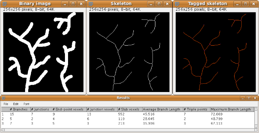 Example of AnalyzeSkeleton performance
|
General Description
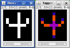 Example of voxel classification
This plugin tags all pixel/voxels in a skeleton image and then counts all its junctions, triple and quadruple points and branches, and measures their average and maximum length. The tags are shown in a new window displaying every tag in a different color. You can find it under Analyze › Skeleton › Analyze Skeleton (2D/3D). See Skeletonize3D for an example of how to produce skeleton images.
The voxels are classified into three different categories depending on their 26 neighbors:
- End-point voxels: if they have less than 2 neighbors.
- Junction voxels: if they have more than 2 neighbors.
- Slab voxels: if they have exactly 2 neighbors.
End-point voxels are displayed in blue, slab voxels in orange and junction voxels in purple.
Notice here that, following this notation, the number of junction voxels can be different from the number of actual junctions since some junction voxels can be neighbors of each other.
Main options
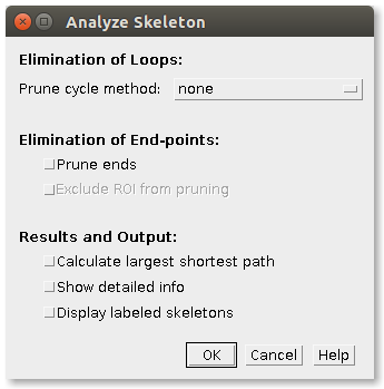 Main dialog of the AnalyzeSkeleton plugin
In the main dialog of the plugin the user can select some options to
- Prune the possible loops in the skeleton (by choosing one of the pruning cycle methods).
- Prune any branch that ends in an end-point (by checking “Prune ends”), as implemented by Michael Doube in BoneJ.
- In this case, if a ROI was selected in the input image, another option is enabled: Exclude ROI from pruning. If selected, pruning will not be applied to end-points contained by the ROI. An application of this feature is described in Strahler Analysis.
- Calculate the largest shortest path of each skeleton using the APSP (all pairs shortest path). In this case, the shortest path will be displayed in a new window containing the skeleton in white and the shortest path in magenta. Implemented by Huub Hovens.
- Show detailed info about the branches of each skeleton in the image.
- Display labeled skeletons. An extra output image will be displayed containing each skeleton labeled with its corresponding skeleton ID.
Loop detection and pruning
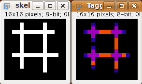 Example of cycle detection and pruning
Since the 2009/09/02 version of the code, the possible cycles or loops in the skeleton can be detected and pruned previous to the analysis. In this sense, the initial plugin dialog offers 4 options:
- none: no cycle detection nor pruning is performed.
- shortest branch: the shortest branch among the loop branches will be cut in its middle point.
- lowest intensity voxel: the darkest voxel among the loop voxels will be cut (set to 0) in the input image.
- lowest intensity branch: the darkest (in average) branch among the loop branches will be cut in its darkest voxel.
For the two last methods, another dialog will pop up asking the user to select the original (gray-scale) image among the open images in order to perform the intensity calculations. The cycle detection is based on a classical “Depth-First Search” (DFS) in the skeleton. The skeleton is treated as an undirected graph, where the end-points and junctions are the nodes and the slab-branches are the edges. While traversing the graph in the DFS fashion, the edges/branches pointing to unvisited nodes are marked as TREE edges, while the edges to visited nodes are marked as BACK edges, which involves the presence of a loop. After the edge classification, the BACK edges are backtracked following their predecessors in order to calculate all the edges belonging to each cycle and proceed with the pruning.
The only known limitation of this approach is shown in the presence of nested loops. In those cases, a second call to the plugin is usually enough to eliminate all the remaining loops.
Table of results
 Example of AnalyzeSkeleton Results table
After classification, a “Results” window is displayed showing for each skeleton in the image:
- The number of branches (slab segments, usually connecting end-points, end-points and junctions or junctions and junctions). The special case of a circular skeleton is also contemplated here.
- The number of voxels of every type: end-point, slab and junction voxels.
- The number of actual junctions (merging neighbor junction voxels) with an arbitrary number of projecting branches.
- The number of triple points (junctions with exactly 3 branches) and quadruple points (4 branches).
- The average and maximum length of branches, in the corresponding units.
AnalyzeSkeleton is able to process up to 231-1 skeletons in one single image (only limited by java Integer.MAX_VALUE).
Detailed information
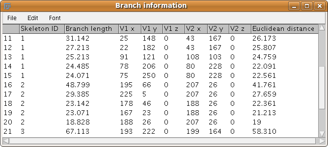 Example of AnalyzeSkeleton Branch information window
When calling the plugin, if the “Show detailed information” checkbox is marked, a complementary results table called “Branch information” is shown.
In this table we display all branches information:
- skeleton ID,
- calibrated branch length,
- 3D coordinates of the extremes of the branch (the so-called V1 and V2 vertices),
- and the Euclidean distance between those extreme points. This value has proven to be a good indicator of the tortuosity of the 3D object.
The branches are sorted by decreasing length.
Video tutorial
For a fast introduction to Skeletonize3D and AnalyzeSkeleton and an example of a real application, you can have a look at this video tutorial.
The tutorial describes step by step how to:
- Pre-process a 3D image to extract the relevant morphological information by
- removing the noise
- and binarizing
- Extract the skeleton of a binary image with Skeletonize3D
- Analyze the resulting skeletons in the 3D image with AnalyzeSkeleton
Visualization
Using the 3D_Viewer libraries we can easily display the results of both, the skeletonization and the analysis:
 Smooth (by 3D Gaussian filter) bat cochlea volume rendered in the viewer
|
 3D skeleton of bat cochlea volume rendered in the viewer after voxel classification
|
 Bat cochlea volume rendered in the viewer with its corresponding classified skeleton
|
Scripting AnalyzeSkeleton
AnalyzeSkeleton functionalities can also be called from scripts, making use of its library methods or performing the whole analysis in silent mode.
Using silent mode from scripts
You can use AnalyzeSkeleton from scripts without displaying any of the results. That’s useful if you want to use the results within the script without the user being annoyed by a lot of results tables popping up.
Here’s an example in Javascript:
importPackage(Packages.ij);
importPackage(Packages.sc.fiji.analyzeSkeleton);

// Takes a binary image as input
var imp = IJ.getImage(); // get current open image

// Skeletonize the image
IJ.run(imp, "Skeletonize (2D/3D)", "");

// Initialize AnalyzeSkeleton_
var skel = new AnalyzeSkeleton_();
skel.calculateShortestPath = true;
skel.setup("", imp);

// Perform analysis in silent mode
// (work on a copy of the ImagePlus if you don't want it displayed)
// run(int pruneIndex, boolean pruneEnds, boolean shortPath, ImagePlus origIP, boolean silent, boolean verbose)
var skelResult = skel.run(AnalyzeSkeleton_.NONE, false, true, null, true, false);

// Read the results
var shortestPaths = skelResult.getShortestPathList().toArray();
var branchLengths = skelResult.getAverageBranchLength();
var branchNumbers = skelResult.getBranches();

var totalLength = 0;
for (var i = 0; i < branchNumbers.length; i++) {
    totalLength += branchNumbers[i] * branchLengths[i];
}

var cumulativeLengthOfShortestPaths = 0;
for (var i = 0; i < shortestPaths.length; i++) {
    cumulativeLengthOfShortestPaths += Number(shortestPaths[i]);
}

// Use the readout within the script
IJ.log(totalLength);
IJ.log(cumulativeLengthOfShortestPaths);
Pruning branches by length
The following Beanshell script prunes the branches of an input skeleton if they are under a certain length:
// @ImagePlus(label="Skeleton image", description="Binary image skeletonized with Skeletonize3D") image
// @double(label="Length threshold", description="Minimum branch length to keep") threshold
// @OUTPUT ImagePlus prunedImage

import sc.fiji.analyzeSkeleton.AnalyzeSkeleton_;
import sc.fiji.analyzeSkeleton.Edge;
import sc.fiji.analyzeSkeleton.Point;
import ij.IJ;

// analyze skeleton
skel = new AnalyzeSkeleton_();
skel.setup("", image);
skelResult = skel.run(AnalyzeSkeleton_.NONE, false, false, null, true, false);

// create copy of input image
prunedImage = image.duplicate();
outStack = prunedImage.getStack();

// get graphs (one per skeleton in the image)
graph = skelResult.getGraph();

// list of end-points
endPoints = skelResult.getListOfEndPoints();

for( i = 0 ; i < graph.length; i++ )
{
    listEdges = graph[i].getEdges();

    // go through all branches and remove branches under threshold
    // in duplicate image
    for( Edge e : listEdges )
    {
        p = e.getV1().getPoints();
        v1End = endPoints.contains( p.get(0) );
        p2 = e.getV2().getPoints();
        v2End = endPoints.contains( p2.get(0) );
        // if any of the vertices is end-point
        if( v1End || v2End )
        {
            if( e.getLength() < threshold )
            {
                if( v1End )
                    outStack.setVoxel( p.get(0).x, p.get(0).y, p.get(0).z, 0 );
                if( v2End )
                    outStack.setVoxel( p2.get(0).x, p2.get(0).y, p2.get(0).z, 0 );
                for( Point p : e.getSlabs() )
                    outStack.setVoxel( p.x, p.y, p.z, 0 );
            }
        }
    }
}

prunedImage.setTitle( image.getShortTitle() + "-pruned" );
Be aware that small branches might be created due to the elimination of end-points and slabs but not junctions (to prevent breaking branches above the threshold). So you might need to run the script a couple of times to remove all unwanted branches.
Visualizing the skeleton in the 3D viewer
The following Beanshell script shows the voxel classification of the skeleton in the 3D viewer:
// @ImagePlus(label="Skeleton image", description="Binary image skeletonized with Skeletonize3D") image

import sc.fiji.analyzeSkeleton.AnalyzeSkeleton_;
import sc.fiji.analyzeSkeleton.Edge;
import sc.fiji.analyzeSkeleton.Point;
import ij.IJ;
import ij3d.Image3DUniverse;
import org.scijava.vecmath.Point3f;
import org.scijava.vecmath.Color3f;

// analyze skeleton
skel = new AnalyzeSkeleton_();
skel.setup("", image);
skelResult = skel.run(AnalyzeSkeleton_.NONE, false, false, null, true, false);

// get calibration
pixelWidth = image.getCalibration().pixelWidth;
pixelHeight = image.getCalibration().pixelHeight;
pixelDepth = image.getCalibration().pixelDepth;

// get graphs (one per skeleton in the image)
graph = skelResult.getGraph();

// create 3d universe
univ = new Image3DUniverse();
univ.show();

// list of end-points
endPoints = skelResult.getListOfEndPoints();
// store their positions in a list
endPointList = new ArrayList();
for( Point p : endPoints )
    endPointList.add( new Point3f(
        (float)( p.x * pixelDepth ),
        (float)( p.y * pixelHeight ),
        (float)( p.z * pixelDepth ) ) );
// add end-points to the universe as blue spheres
univ.addIcospheres( endPointList, new Color3f( Color.BLUE ), 2, 1f, "End-points");

// list of junction voxels
junctions = skelResult.getListOfJunctionVoxels();
// store their positions in a list
junctionList = new ArrayList();
for( Point p : junctions )
    junctionList.add( new Point3f(
        (float)( p.x * pixelDepth ),
        (float)( p.y * pixelHeight ),
        (float)( p.z * pixelDepth ) ) );
// add junction voxels to the universe as magenta spheres
univ.addIcospheres( junctionList, new Color3f( Color.MAGENTA ), 2, 1f, "Junctions");

for( i = 0 ; i < graph.length; i++ )
{
    listEdges = graph[i].getEdges();

    // go through all branches and add slab voxels
    // as orange lines in the 3D universe
    j=0;
    for( Edge e : listEdges )
    {
        branchPointList = new ArrayList();
        for( Point p : e.getSlabs() )
            branchPointList.add( new Point3f(
                (float)( p.x * pixelDepth ),
                (float)( p.y * pixelHeight ),
                (float)( p.z * pixelDepth ) ) );
        // add slab voxels to the universe as orange lines
        univ.addLineMesh( branchPointList, new Color3f( Color.ORANGE ), "Branch-"+i+"-"+j, true );
        j++;
    }
}
API documentation
The latest documentation of the code can be found here:
http://javadoc.imagej.net/Fiji/sc/fiji/analyzeSkeleton/package-summary.html
Changelog
All changes can be seen in the GitHub source repository.
2010/12/28: Jan Eglinger added code to call the plugin from script in silent mode.
2010/09/27: Added Huub Hovens’s code to detect the shortest largest path in each skeleton and Michael Doube’s code to prune the branches ending on end-points.
2010/08/26: Fixed bug that was assigning wrong final vertices (V2) to the edges when visiting the trees from end-points if the branches were ending on already visited junctions. Reported by Peter C. Marks.
2010/01/12: Thanks to Peter Marks, fixed bug to visit properly the trees when starting in junctions (they were not being added to the revisit list, what some times made some trees to be split).
2009/12/04: Added quadruple point calculation.
2009/09/13: Removed Log window and created Detailed information option and Branch information table.
2009/09/02: Added capability to detect and prune skeleton cycles.
2009/08/10: Fixed small bug to treat the special case of one single circular skeleton.
2009/08/06: Fixed 2 bugs: calculation of branches between junctions and number of slab voxels in a circular tree.
2009/08/05: Fixed bugs that slowed down the calculation of the number of actual junctions.
2009/06/19: Fixed bugs in some calculations, increased the number of skeletons from 255 to 2¹⁵-1, and added new (previously untreated) cases.
2009/04/07: Added different calculations for every skeleton in the image and some extra information in the log window.
2009/03/05: Added maximum branch length calculation.
2008/11/19: Added triple points calculation and fixed bug to avoid modifying the original image and preserve its calibration in the output image.
2008/11/16: First release.
References and citation
If you need to cite the plugin, please do so by citing the following paper:
The shortest path calculation and its applications have been published as:
- G. Polder, H.L.E Hovens and A.J Zweers, Measuring shoot length of submerged aquatic plants using graph analysis (2010), In: Proceedings of the ImageJ User and Developer Conference, Centre de Recherche Public Henri Tudor, Luxembourg, 27-29 October, pp 172-177.
AnalyzeSkeleton makes also part of BoneJ, a plugin for bone image analysis in ImageJ:
- Michael Doube, Michal M. Klosowski, Ignacio Arganda-Carreras, Fabrice P. Cordelieres, Robert P. Dougherty, Jonathan S. Jackson, Benjamin Schmid, John R. Hutchinson, Sandra J. Shefelbine, BoneJ: Free and extensible bone image analysis in ImageJ, Bone, Volume 47, Issue 6, December 2010, Pages 1076-1079.
License
This program is free software; you can redistribute it and/or modify it under the terms of the GNU General Public License as published by the Free Software Foundation (http://www.gnu.org/licenses/gpl.txt).
This program is distributed in the hope that it will be useful, but WITHOUT ANY WARRANTY; without even the implied warranty of MERCHANTABILITY or FITNESS FOR A PARTICULAR PURPOSE. See the GNU General Public License for more details.