Learn to analyze sub-areas of an image

What is a sub scan?

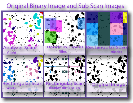
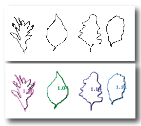
This page tells how to do and interpret a sub scan, which is a regular box counting scan applied to potentially many individual local areas of an image. The pictures below, which include graphics files generated as part of a sub scan, show the general idea of sub scanning.

If you need to know the basics behind setting up a scan in general, go to the basic tutorial. For information on how to set up colour coding for the scanning described on this page, go here. For LCFD or local connected fractal dimension scans, click here.

Sub scans show how locally calculated fractal dimensions are distributed in an image and how they depend on sample size. The images above illustrate the basic outputs of the two major types of subscan - particle analyzer and rectangular. The binary contours were automatically found by running a FracLac scan that invokes the ImageJ particle analyzer on one image as shown, then analyzes the detected particles as separate bodies.

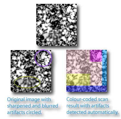
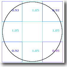
The others were rectangular scans. The grayscale texture was systematically scanned in blocks. That scan automatically detected two areas of difference in the texture, which are artifacts created using blurring and sharpening in ImageJ on ROIs on the original image. The artifacts are circled on the lower image. The results of the scan, the colour coded blocks, show the corresponding general areas where the differences were found as a difference in the local DBGray. The simple binary circle was scanned with a rectangular scan, to illustrate local variation attributable to digitization.

Results Files

In addition to graphics files like those you saw above, a sub scan generates results files. The main results file of a sub area scan is the same file as from a regular scan, except that it contains several rows for each image, corresponding to several samples taken during the sub area scan.
To interpret the results file from a subscan, see the main Results file page.

The screen shot below shows the options panel for a sub scan. Click on a part of the image or scroll past the image to the listings to find out what the settings are for and how to interpret their results.
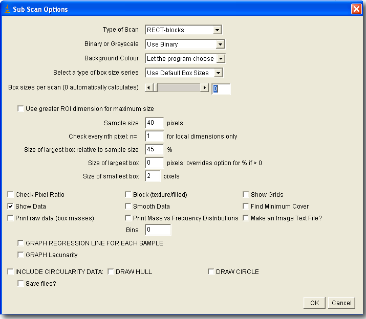
Type of Scan

Select the way to sample the image and present the data from this drop-down menu. For setting colour options, go to the Colour Selection Page.

    The general type of scan is:
  1. LOCAL (not connected): this scans pixels by pixel, so can be very slow. It determines the mass dimension around every nth pixel horizontally and vertically, so is very sensitive to this setting.
  2. ANALYZER: Uses ImageJ's built-in Particle Analyzer, ignoring the settings for sample size; size and other options are set in the dialog for the particle analyzer (see IJ documentation).
  3. RECTANGULAR: Samples the image using a rectangular array of squares, using the sample size selected on the panel.
  4. RANDOM: samples square areas, as many as the number chosen in a popup that appears when you choose this option, using the sample size selected on the panel. As illustrated in the images below, this option can overlap whereas the rectangular cannot.
    The display types are illustrated in the image:
  1. contour shows the contour of the area scanned, colour-coded according to the DB of the area
  2. display dimension prints the DB itself
  3. fill/pixels colours foreground pixels according to the DB for the area.

Draw Hull

Select to generate a file for Hull Metrics and the Convex Hull

Draw Circle

Select to generate a file for Hull Metrics and the Bounding Circle

Include Circularity Data

Select to generate a file for Hull Metrics

Graphs

Graph Regression Line for Each Sample

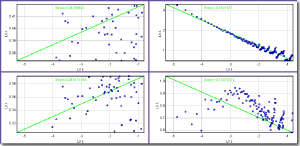
Select to generate graphs showing regression lines and data for the DB for each subsample; note that this can generate a very high number of graphs (see Saving files automatically).

Graph Lacunarity

Select to generate graphs showing lacunarity for each subsample; note that this can generate a very high number of graphs (see Saving files automatically).

Bins for Frequency Distributions

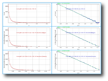
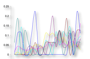
Type a number for the number of bins to use for the mass vs. frequency distribution for pixel mass (one distribution for each ε for each sample), which is used to calculate BPD lacunarity; if this is 0, then no frequency distribution data are generated. This option generates a data file; the image below illustrates a graph of the data for pixel mass at each ε showing the binned frequency distributions from one sample..

Make an IMAGE Text File

Select this option to make an image txt file that ImageJ can open, with the colour-coding as a single DB for each area

Print Mass vs Frequency Distributions

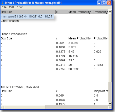
Select this option to generate a data file with the binned probability distribution for pixel masses. Note that if the number of bins is less than 1, this option is ignored. As highlighted on the screen shot of the file shown below, a file with the ROI location and size printed on the first line is generated for each sample. Click here for more on interpreting the file.

Print raw data (box masses)

See explanation in regular box counting

Save files automatically.

See explanation in regular box counting

Filters

Use Smoothing Filter

See explanation in regular box counting

Find Minimum Cover

See explanation in regular box counting

Show Data

See explanation in regular box counting

Sizes

Size of Smallest box

See explanation in regular box counting

Size of largest box

See explanation in regular box counting

Size of largest box relative to sample size

See explanation in regular box counting

Check every nth pixel n=

For local dimension scans only, scans only at every nth pixel instead of every pixel.

Sample size

Type a number for the size of the sample, as the side of a square in pixels, for rectangular scan types. This option is ignored and the sample size is set separately for particle analyzer scans.

Doing subscans takes considerably more time for 1) larger images and 2) smaller subscan sample sizes.

Use greater ROI dimension for maximum size

See explanation in regular box counting

Box sizes per scan (0 automatically calculates)

See explanation in regular box counting

Select a type of box size series

See explanation in regular box counting

Colour

Background Colour

See explanation in regular box counting

Binary of Grayscale

See explanation in regular box counting

Show Grids

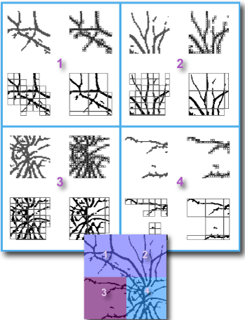
Select this option to make a stack of images showing the series of boxes laid on each sample, for boxes that contained foreground pixels and were counted. As illustrated in the image below, this option mkaes a stack of images for each sample, which could lead to a large number of files (see Saving Files Automatically).(For this image, each stack was converted to a montage using Image»Stacks»Make Montage in ImageJ on the stacks generated by selecting this option while doing a subscan for the image shown at the bottom with the sample size set so that 4 samples were used.)

To learn how to make images showing grids used, try the grid generating tutorial.

Block (texture/filled)

See explanation in regular box counting

Check Pixel Ratio

See explanation in regular box counting