Are you experiencing deep consternation over an image you know must have hidden areas of significance that will be objectively revealed by fractal analysis?
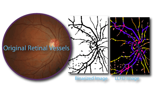
Does the illustration showing my retinal vessels, a binarized version of the image, and a colour-coded scan result automatically highlighting certain areas look like what you need? Then this might be the place to find inner peace.
The basic premise of a local connected fractal dimension (LCFD) scan is that we can identify meaningful local variation in complexity...and even present it visually!
Landini's paper applying
LCFD analysis to the diagnosis of retinal vascular disease is a great reference for the technique. FracLac implements his basic ideas and this page shows you how it all works.
Are you ready to build on your earlier background and learn how to set up and interpret an LCFD analysis?
- Using this Page:
- Setting Options:
- Click various options on the screenshot
- Scroll down or jump to the whole list.
- General Knowledge:
- See the Tips section of this page
- or see the BoxCounting page.
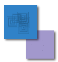
This page is the practical reference for Local Connected Fractal Dimension or LCFD scans.If you are looking for something similar and think you arrived at the wrong page, try the Sub Scans page.
The page assumes you are familiar with the basics of using FracLac, are grounded in connected sets, know how LCFD scanning methods (illustrated in the image above) differ from regular box counting, and want to learn more about setting the options and interpreting the results from LCFD scans.
Options
To learn about options, click on them on the screenshot, which is an image of the basic options panel that comes up when you select a LCFD scan in FracLac. If you prefer, scroll down to the list.
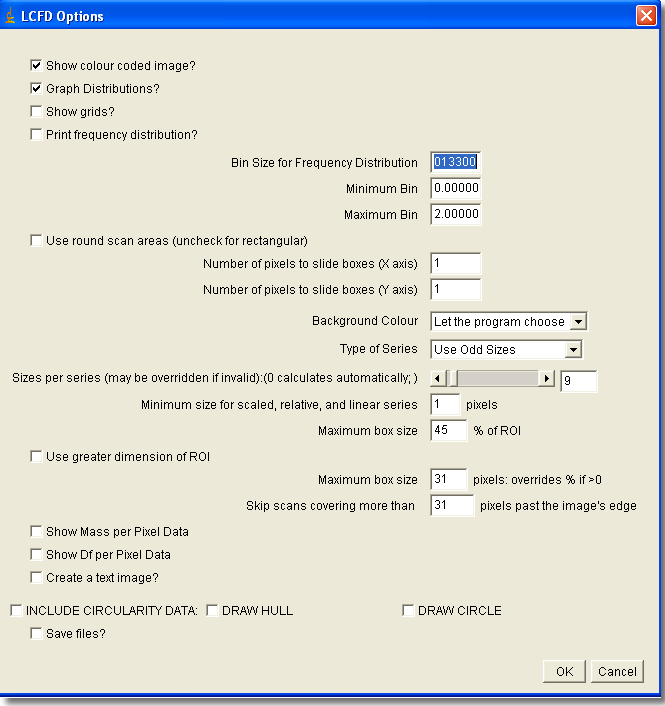
The Options
Tips
DF Distributions
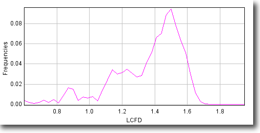
To help determine a suitable range for colour-coding, you can generate a data file as well as a graphics file of how the LCFD was distributed over an image. There are 3 parameters to set for the distribution itself—the minimum, maximum, and bin size or increment between DFs. The default is from 0 to 2 with a binsize of 0.0133; however, these numbers should reflect the numbers you expect to see in the images you are analyzing, and you may wish to do trial runs to determine a particular range. See the colour-coding tip for more information.
Colour Coding
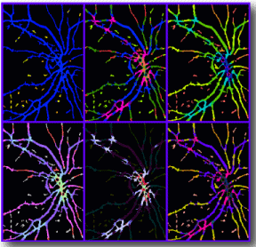 With the colour-coding option selected, you can view the same data
set in different ways, adjusting the colours to accentuate areas
with a certain range of LCFD values. In other words, the picture
of retinal vessels
you saw above
is not all there is to LCFD scans.
This montage shows the results of one scan on one image, with
multiple LUTs
applied when the scan was done. Each LUT highlights different aspects of
the distribution of LCFDs (e.g., compare the right central area of all
of the images).
You can colour-code any LCFD scan on screen or as a batch job, and can view the results on screen or save them automatically to a folder.
Prior to scanning batch jobs, you may want to know what range of fractal dimensions your images will show variation over. You can determine this by doing a scan on a single slice on screen, which will show a popup letting you modify the results in real time. This option is not available for batch jobs and stacks with more than 1 slice.The coloured graphic of your original image will appear showing the LCFD at each pixel along with a legend showing what each colour means. A dialog asks if you would like to try another LUT (another set of colours and/or associated codes). You may choose to do it many, many times with one image as, for example, you home in on the areas in the image that trouble you most. See the distribution tip for more on this issue.
Use the Frequency Distribution to help determine the best range.
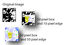 This setting sets a margin around the scanning area. The image illustrates a scan using a 50 pixel maximum box size with the area to skip set at 10 pixels and at 50 pixels. Use this setting to avoid sampling edges when that will adversely affect your results. You may need to explore how the maximum box size and the margin interact for different types of images.
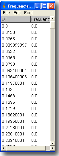 The screen shot shows the contents of the file - a column for the LCFD and one for the frequency of each value.