Sholl Analysis
| Sholl Analysis | |
|---|---|
| Project | Fiji |
| URL | https://imagej.net/Sholl |
| Source | on GitHub |
| License | GPLv3 |
| Release | 3.6.12 |
| Date | Mon Jan 16 23:02:41 CST 2017 |
| Development status | Active |
| Support status | Active |
| Team | |
| Founders | Tom Maddock |
| Leads | Tiago Ferreira |
| Developers | Tiago Ferreira |
| Debuggers | Tiago Ferreira |
| Reviewers | Tiago Ferreira |
| Support | Tiago Ferreira |
| Maintainers | Tiago Ferreira |
| Contributors | Tom Maddock, Mark Hiner, Curtis Rueden, Johannes Schindelin |
- Analysis of traced arbors?
- Jump to Traced Cells or Other tracing software
- Segmentation issues?
- Jump to Cf. Segmentation or Pre-processing
- Having Problems?
- Jump to FAQs
Contents
- 1 Introduction
- 2 Installation
- 3 Direct Analysis of Images
- 4 Analysis of Traced Cells
- 5 Analysis of Existing Profiles
- 6 Parameters
- 7 Sholl Plots
- 8 Metrics
- 9 Complementary Tools
- 10 Pre-processing
- 11 Batch Processing
- 12 Advanced Usage
- 13 Auxiliary Commands
- 14 FAQ
- 15 Release Notes and Pre-releases
- 16 Related Resources
- 17 Publication
- 18 Citations
- 19 References
- 20 License
Automated and multithreaded Sholl for direct analysis of fluorescent images and traced morphologies. Features powerful quantifications based on curve fitting. Analysis of data obtained outside of ImageJ is also possible.
Introduction
The Sholl technique[2] is used to describe neuronal arbors. This plugin can perform Sholl directly on 2D and 3D grayscale images of isolated neurons. Its internal algorithm to collect data is based upon how Sholl analysis is done by hand — it creates a series of concentric shells (circles or spheres) around the focus of a neuronal arbor, and counts how many times connected voxels defining the arbor intersect the sampling shells. The major advantages of this plugin over other implementations are:
- When analyzing images directly, it does not require previous tracing of the arbor (although it can also analyze traced arbors)
- It combines curve fitting with several methods to automatically retrieve quantitative descriptors from sampled data, which allows direct statistical comparisons between arbors
- It allows continuous and repeated sampling around user-defined foci
- It allows batch processing
Installation
The plugin is distributed with Fiji. It installs several commands under Analysis ▷ Sholl ▷ . As part of an active effort to modernize ImageJ you need to subscribe to the Java 8 update site to access the latest plugin version (this will also allow you to access the newest ImageJ capabilities). To do so, you can either:
- Download the latest Fiji release. Newer releases come pre-bundled with Java 8, and are already subscribed to the Java-8 update site.
- If you have downloaded Fiji while ago and want to keep your existing installation, you will have to download Java 8 and make your Fiji installation aware of it. Then subscribe to the Java-8 update site.
Direct Analysis of Images
In this mode (bitmap analysis), the plugin requires a binary image or a segmented grayscale image (2D or 3D) containing a single neuron.
- Segment the neuronal arbor using Image ▷ Adjust ▷ Threshold... (shortcut: ⇧ Shift+T ).
- N.B.: When using multichannel images, you will have to set the its display mode to Grayscale using Image ▷ Color ▷ Channels Tool... (⇧ Shift+Z), because images displayed as Composites cannot be thresholded.
- Define the center of analysis using a valid startup ROI.
- Run Analysis ▷ Sholl ▷ Sholl Analysis..., adjusting the default Parameters in the dialog prompt.
- Press More » Cf. Segmentation to visually inspect the two thresholded phases: arbor and background.
- Problems? Read the FAQs.
Startup ROI
The center of analysis can be specified using one of three possibilities:
- Straight line
- A Straight line from the focus of the arbor to its most distal point using the Straight Line Tool. The advantages of using line selections are twofold: 1) Center of analysis and Ending radius are automatically set, and 2) Horizontal/vertical lines (created by holding ⇧ Shift while using the Straight Line Selection Tool) can be used to restrict analysis to sub-regions of the image.
- Single point
- A single point marking the focus of the arbor using the Point Selection Tool. With single point selections, only the center of analysis is defined. Thus, this option is suitable for batch processing of images with different dimensions with undefined Ending radius.
- Multi-point selection
- A Multi-point selection (multi-point counter) in which the first point marks the center of analysis while the remaining points mark (count) the number of primary branches required for the calculation of ramification indices). Suitable for cases in which inference from starting radius is not effective.
Cf. Segmentation
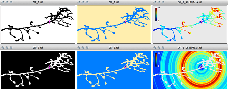
Press More» Cf. Segmentation to visually confirm which phase of the segmented image will be sampled. This command highlights foreground from background pixels and is particularly useful when analyzing black and white (binary) images or when using the B&W lookup table in the Threshold Widget (Image▷ Adjust▷ Threshold... ⇧ Shift+T). Cf. Segmentation allows you to ensure that you are measuring neuronal processes and not the interstitial spaces between them. Here is an example using an axonal arbor of a Drosophila olfactory neuron from the DIADEM dataset[3]:
Note the reversal of Cf. Segmentation output and how the intersections mask no longer decorates the axonal processes but the interstitial spaces between them. The consequences of the phase inversion are twofold: 1) the program oversamples (cf. hue ramps on upper left of Intersections mask) and 2) the program detects artifacts induced by the edges of the image (cf. top-right and bottom-right corners of mask where intersections are sampled in the absence of real axons at those locations). Also, note that the initial black and white image would look the same under an inverted lookup table (Image ▷ Lookup Tables ▷ Invert LUT). |
Analysis of Traced Cells
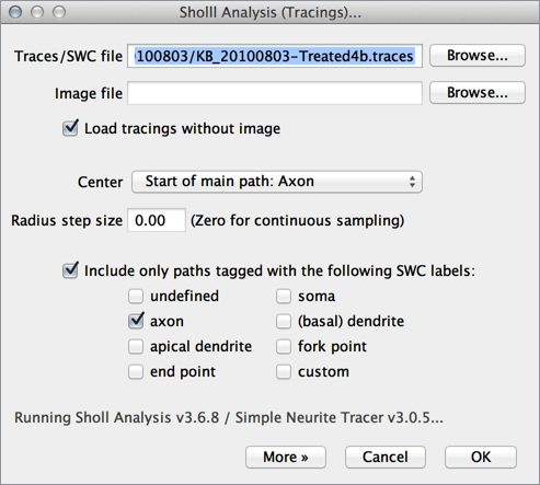
In this mode, the plugin analyzes reconstructed arbors. This is particularly relevant for stainings that do not allow single-cell resolution. The plugin is macro recordable and batch processing is also possible.- Run Analysis ▷ Sholl ▷ Sholl Analysis (Tracings)... and specify a tracing file (a
.swc, a.eswcor a Simple Neurite Tracer.tracesfile). If you want, you can also specify the image associated with the reconstruction. This will allow the plugin to use the image's metadata to determine spatial units and x,y,z spacing. - Choose the center of analysis using the drop down menu in the main prompt listing SWC tags (axon, dendrite, soma, etc.). Note that if your tracings are not tagged you can do so in Simple Neurite Tracer
- Adjust the default Parameters
- Problems? Read the FAQs
Analysis of Existing Profiles
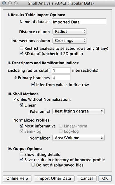
This feature is processed by Analysis ▷ Sholl ▷ Sholl Analysis (Existing Profile).... This command can be used to re-analyze data (replot, modify fitting options, etc.) without having to access the initial image or tracing data. Batch processing is also possible. Noteworthy:
- Input data: Any tab or comma delimited text file (.csv, .txt, .xls, .ods) can be used. You can drag & drop these files into the main ImageJ window, import data from the clipboard, or use data from any other table already opened by ImageJ.
- Restricting input data: To restrict measurements to a range of distances (see related example), select the range of distances you want analyze. You can click the first row in the range, and then drag the mouse to the last row, or by holding down ⇧ Shift while selecting the last row in the range. Then, in the prompt, activate the Restrict analysis to selected rows only checkbox.
- Calculation of Radius step size: Radius step size is calculated from the difference between the first two rows in Distance column. This is mainly relevant when choosing Annulus/Spherical shell as normalizer.
Parameters
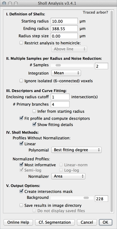
The majority of parameters is shared by all the Analysis commands in theAnalysis ▷ Sholl ▷ submenu. However, some settings are specific to the type of data used as input: A segmented image, a tracing, or a previously obtained profile. When analyzing images, input values take into account the scale information of the image (which can be set using the Analyze ▷ Set Scale... or Image ▷ Properties... (⇧ Shift+P), the type of image (2D or 3D), and its active ROI.
Definition of Shells
- Starting radius The radius of the smallest sampling circle/sphere, i.e., the first distance to be sampled.
- Ending radius The radius of the largest (last) sampling circle/sphere. It is automatically calculated if a line ROI is used. Note that the specified distance may not be actually sampled, if Radius step size is not a divisor of Ending radius-Starting radius. In this case, the program will choose the largest possible distance smaller than the specified value.
N.B. You can clear Ending radius or set it to NaN ("Not a Number") to sample the entire image. This is particularly useful when batch processing images with different dimensions.
- Radius step size The sampling interval between radii of consecutive sampling circles/spheres. This value may be set to zero for continuous (1-voxel increment) measurements.
N.B. For stacks with anisotropic voxel size, setting Radius step size to zero, sets the step length to the dimension of the matching isotropic voxel, i.e., the cube root of the product of the voxel dimensions (3D images) or the square root of the product of the pixel dimensions (2D images).
- Restrict analysis to hemicircle/hemisphere This option is only available when an orthogonal radius has been created (by holding ⇧ Shift while using the Straight Line Selection Tool). It can be used to limit the analysis to sub-compartments of the arbor.
N.B. For horizontal lines, this option instructs the algorithm to measure intersections at sites equidistant from the center that have y-coordinates above/below the drawn line. For vertical lines, it instructs the plugin to measure intersections at sites equidistant from the center that have x-coordinates to the left/right of the drawn line.
Multiple Samples/Noise Reduction
- Samples per radius (2D images only) Defines the number of measurements to be performed at each sampling circumference. These measurements are then combined into a single value according to the chosen integration method. This strategy, a break from previous approaches, increases the accuracy of non-continuos profiles by diluting out the effect of processes extending tangent to the sampling circumference.
- Visually, this option can be imagined as the "thickness" of the sampling circumference: e.g., for a radius of 100 pixels and a value of 3 Samples per radius, the final number of intersections would integrate the measurements sampled at distances 99, 100 and 101.
- Note that it would not make sense to increase the number of samples beyond the length (in pixels) of Radius step size. For this reason, this option is limited to a draconian (and arbitrary) maximum of 10 samples.
- Samples integration (2D images only) The measure of central tendency used to combine intersection counts when multiple Samples per radius are used. Options are Mean (the default), Median or Mode.
- Ignore isolated (6-connected) voxels (3D images only) If checked, single isolated voxels intersecting the surface of sampling spheres are not taken into account, which may allow for smoother profiles on noisy image stacks. However, it should be noted that connectivity in the stack volume may not reflect connectivity on the surface of a digitized sphere. Indeed, in certain contexts, it is possible (though unlikely) to obtain higher intersection counts when this filtering option is active.
- Please keep in mind that this is just a refinement feature, and you should not expect it to mitigate the effects derived from poorly-segmented arbors.
Descriptors and Curve Fitting
- Enclosing radius cutoff The number of intersections to be used in the definition of Enclosing radius.
- Number of primary branches The number of primary branches (i.e., those originating directly from cell soma when the center of analysis is the perikaryon) to be used in the calculation of Schoenen ramification indices. It is automatically populated using multi-point counts if a multi-point ROI is detected at startup. Set it to zero (or NaN) to disable calculations of ramification indices.
- Infer from starting radius If checked, the Number of Primary branches is inferred from the count of intersections at Starting radius.
- Fit profile and compute descriptors If checked, data is fitted according to the chosen method and appropriate metrics calculated automatically. If unchecked, only sampled data is plotted.
- Show fitting details Choose this option to have all of the parameters of the simplex fitting printed to the Log window. The coefficient of determination (R2, a measure of goodness of fit) is always stored in the Sholl Results table even when this option is not selected.
Choice of Methods
The type of profile(s) to be obtained. Linear (profile without normalization), or normalized profiles: Linear-norm, Semi-log, or Log-log.
- Polynomial Specifies the degree of the polynomial to be fitted to the Linear profile[4]. While the polynomial of best approximation, or "best fit", should be empirically determined for each analyzed cell type, it is possible to ask the plugin to predict the order of the fitting polynomial (or at least try) using the choice Best fitting degree. In this case, the plugin will loop through all the available choices of polynomials, perform each fit in the background and choose the one with the highest coefficient of determination.
- Most informative Select this option when you cannot predict which type of normalized profile best describes the dataset. If chosen, the plugin will use the Determination ratio to determine which of Semi-log or Log-log methods is more appropriate. Linear-norm is not performed.
The Best fitting degree and Most informative choices are obviously more computer-intensive and can be monitored by activating the Show fitting details checkbox. - Normalizer The property of the sampling shell to be used in the normalization of Linear-norm, Semi-log, and Log-log profiles. It is described below.
Output Options
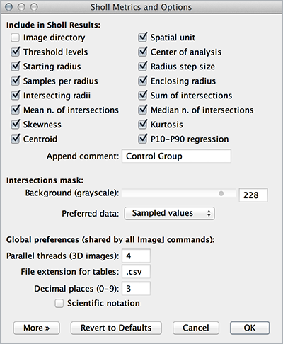
- Create intersections mask If checked, a 16/32–bit maximum intensity projection of the analyzed image is generated in which the measured arbor is painted according to its Sholl profile. The type of data (Raw, i.e., sampled or Fitted) is displayed in the image subtitle and can be specified in Analysis ▷ Sholl ▷ Metrics & Options... or using the Options... command in the More» drop-down menu.
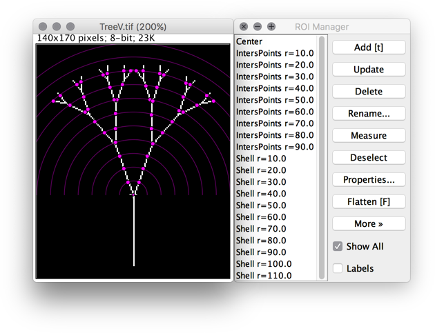
NB: The default Lookup Table (LUT) used by the mask can be changed using Image ▷ Lookup Tables. The background color [gray level: 0 (black) to 255 (white)] can also be set in Metrics & Options..., or at any later point using Image ▷ Color ▷ Edit Lut... WYSIWYG versions (RGB images) of these masks can be otained using by pressing ⇧ Shift+F (Image ▷ Overlay ▷ Flatten) or by running Analyze ▷ Tools ▷ Calibration Bar... - Overlay sampling shells and intersection points (2D images only) If checked, two sets of ROIS are added to the image overlay: 1) concentric shells matching sampled distances (circular ROIs or composite ROIs when using hemicircles); and 2) Multipoint ROIs at intersection sites between shells and clusters of foreground pixels.
- Save results to If checked, all the results (with the exception of the Sholl Table) are saved to the specified directory. These include: 1) Sholl plots (saved as PNG images), 2) A table containing detailed data and 3) The Sholl mask. Files are named after the image filename and analysis method. Saving options can be specified in Analysis ▷ Sholl ▷ Metrics & Options... (Options... command in the More» drop-down menu).
- Do not display saved files If checked, saved files are directly saved to disk and are not displayed. Activate this option when batch processing files.
Sholl Plots
Linear, Linear-norm, Semi-log and Log-log profiles for the ddaC cell (File ▷ Open Samples ▷ ddaC Neuron), version 3.0. Most of the retrieved metrics are automatically highlighted by the plugin. Linear profile: Mean value (horizontal grid line) and Centroid (colored mark). Logarithmic profiles: The Sholl regression coefficient (also known as Sholl decay) can be retrieved by linear regression using either the full range of data (blue line) or data within percentiles 10–90 (red line). For this particular cell type, the Semi-log method is more informative when compared to the Log-log method.
| Method | Fit | Description | |
|---|---|---|---|
| (1) | Linear | N = a + br + cr2 + dr3 + er4 + fr5 + ... + xrn | Outputs a N vs Distance profile. Data is fitted to a polynomial function[4]. Critical radius, Critical value and Mean value of function are calculated |
| (2) | Linear-norm | N/S = a rb | Outputs a N/S vs Distance profile. Points are fitted to a power function. It is an intermediate representation of the data that can be used to gauge the choice of normalizer. Once plotted under a logarithmic scale the Linear-norm curve is similar to the Semi-log profile |
| (3) | Semi-log | log(N/S) = -k r + m | Outputs a log(N/S) vs Distance profile. A linear regression is fitted to the sampled data. The Sholl regression coefficient (k) is calculated |
| (4) | Log-log | log(N/S) = -k × log(r) + m | Outputs a log(N/S) vs log(Distance) profile. Data is also fitted to a straight line. This is an alternative approach[5] of obtaining a relevant regression coefficient, when the Semi-log method returns a poor fit |
N For 2D images, the Number of clusters of pixels (8–connected) intersecting the circumference of radius r
For 3D images, the Number of clusters of voxels (26-connected) intersecting the surface of the sphere of radius r
r Distance from center of analysis (radius of Sholl circle/sphere)
log Natural logarithm, the logarithm to the base e
SThe chosen property of the sampling shell to be used in the normalization of Linear-norm, Semi-log, and Log-log profiles.
For 2D images, the Perimeter of the sampling circumference (2πr) or the Area of the corresponding circle (πr2)
For 3D images, the Surface of the sampling sphere (4πr2) or its respective Volume (4/3πr3)
N.B. A third normalization option is also available when performing non-continuous sampling: Annulus/Spherical shell. In this case, the normalization is performed against the area of the annulus formed between the circumferences at r ± Radius step size/2 (2D images), or against the volume between the two spheres at r ± Radius step size/2 (3D images).
Metrics
Morphometric descriptors and other properties of the arbor are printed to a dedicated table named Sholl Results. Output is fully customizable using Analysis ▷ Sholl ▷ Metrics & Options... or using the Options... command in the More» drop-down menu. The first columns log analysis parameters: Image Directory, filename and voxel unit, Channel, Lower and Upper Threshold levels, X,Y (in pixels) and Z (slice number) coordinates of center of analysis, Starting and Ending radius, Radius step, Number of Samples per Radius, etc. Other parameters are described below.
Metrics based on sampled data
- Intersecting radii
- The number of sampling radii intersecting the arbor at least once.
- Sum of intersections (Sum inters.)
- The sum of all intersections.
- Mean of intersections (Mean inters.)
- Sum inters. divided by Intersecting radii.
- See also Mean value, FAQ
- Median of intersections (Median Inters.)
- The median value of sampled intersections.
- Skewness
- The skewness of the sampled data, an indication of how symmetrical the distribution is around its mean. Positive values indicate an asymmetrical distribution with a longer tail to the right. Negative values indicate data with a longer tail to the left. A popular rule of thumb considers that if the skewness is greater than 1.0 (or less than -1.0), the distribution may be considered far from symmetrical.
- See also Skewness (fitted data)
- Kurtosis
- The kurtosis of the sampled data, which quantifies whether the shape of the distribution matches that of a Gaussian distribution, assuming that a Gaussian distribution has a kurtosis of 0. A distribution more peaked than a Gaussian has a positive kurtosis while a negative value indicates a flatter distribution.
- See also Kurtosis (fitted data)
- Highest count of intersections (Max inters.)
- The maximum value of sampled intersections, i.e., the maximum in a linear [N vs Distance] profile, reflecting the highest number of processes/branches in the arbor.
- See also Critical value
- Radius of highest count of intersections (Max inters. radius)
- The distance at which the Highest count of intersections occurred, reflecting sites of highest branch density. Note that if the same maximum occurs multiple times, only the first distance is considered.
- See also Critical radius
- Schoenen Ramification index (Ramification index (sampled))
- A measure of ramification[6]: the ratio between Max inters. and the number of primary branches. It is only calculated when primary branches is valid and not zero.
- See also Ramification index (fit)
- Centroid radius
- The abcissa of the centroid (i.e., the geometric center or barycenter) of the linear profile. It is highlighted on the N vs Distance plot.
- Centroid value
- The ordinate of the centroid (i.e., the geometric center or barycenter) of the linear profile. It is highlighted on the N vs Distance plot.
- Enclosing radius
- The last (thus, the widest) of Intersecting radii to be associated with the number of intersections specified by Enclosing radius cutoff. For a cutoff of 1 (the default) Enclosing radius is the widest of Intersecting radii. It reflects the Feret length of the arbor.
Metrics based on fitted data
- Determination ratio
- The ratio of the coefficient of determination for the semi-log method and that for the log–log method[5]. If the semi-log method is better relatively to the log–log method, the Determination ratio becomes larger than 1. It is the parameter used by the plugin to silently predict the normalization method that is the most informative. The prediction can be monitored by activating the Show fitting details checkbox.
- Sholl regression coefficient (Regression coefficient)
- The slope (multiplied by -1) of the linear regression described in (3) and (4), i.e., k, a measure of the rate of decay of the number of branches with distance from the center of analysis. Higher k values reflect larger changes in the function log(N/S). To optimize the fit, the plugin retrieves a second linear regression centered around the median distance, excluding distances at the edges of the profile. Details of this second fit are also registered on the Sholl table under dedicated columns, e.g., Sholl regression coefficient [P10-P90], when data within the 10th–90th percentile is used.
- Regression R2 (Regression R^2)
- The coefficient of determination of the linear regression described in (3) and (4).
- Critical value
- The local maximum of the polynomial fit, i.e, N at Critical radius in (1). Abbreviation: Nm.
- See also Max inters.
- Critical radius
- The distance at which Critical value occurs. By default (see Advanced Usage), it is calculated with a precision of 1/1000 of Radius step size. Abbreviation: rc.
- See also Max inters. radius
- Mean value
- The mean value[4] of the fitted polynomial function (1), representing the average of intersections over the whole area occupied by the arbor. Abbreviation Nav.
- On the Sholl plot, it is highlighted as the height of the rectangle that has the width of Enclosing radius − First intersecting radius and the same area of the area under the fitted curve on that discrete interval. It is analogous to Mean inters., the arithmetic mean of sampled intersections throughout the arbor (cf. Metrics based on sampled data). By default (see Advanced Usage), it is calculated with a precision of 1/1000 of Radius step size.
- Schoenen Ramification index (Ramification index (fit))
- Schoenen Ramification index retrieved from fitted profile: The ration between Critical value and Number of primary branches.
- See also Ramification index (sampled)
- Skewness (Skewness (fit))
- The skewness of the fitted polynomial distribution between Starting radius and Ending radius.
- Kurtosis (Kurtosis (fit))
- The kurtosis of the fitted polynomial distribution between Starting radius and Ending radius.
- Polynomial R2 (Polyn. R^2)
- The coefficient of determination of the polynomial fit described in (1).
Complementary Tools
Sholl Analysis tries to be as flexible as possible by providing several options for normalization and curve fitting. However, it cannot offer exhaustive curve fitting options as determining best fit models requires reasonable choices that are not amenable to full automation. For this reason, complementary tools for curve fitting can be installed as needed using BAR by subscribing to its update site. Several BAR commands complement Sholl Analysis. These include:
- Segmentation tools
- Thresholding, shape-based masking and edge-detection routines (see full BAR list)
- Data analysis tools
- Find Peaks: Retrieves local maxima under several filtering options such as peak amplitude, peak height and peak width. Can be used to retrieve secondary sites of branch density
- Fit Polynomial: Fits a polynomial of any degree to sampled data. Features an heuristic algorithm for guessing a polynomial "best fit". Expands the built-in repertoire of polynomial fits up to 50th order functions.
- Create Boxplot: Allows direct comparison of metrics between groups or sets of data (specially useful when tagging images with the Comment field in Analysis ▷ Sholl ▷ Metrics & Options...)
- Interactive Plotting: Whole-purpose routine that plots data from imported spreadsheets.
Pre-processing
This section discusses some aspects that should be taken into account when segmenting neuronal arbors to be processed by Sholl Analysis. Since image segmentation (i.e., the partitioning of images into analyzable parts) is vulnerable to noise and background fluorescence, it is not possible to generalize universal routines that efficiently binarize grayscale images. This means that any procedure that tries to appropriately describe the original fluorescence image with a binary mask must be tailored to the characteristics of individual datasets. As mentioned in Complementary Tools, several routines listed here as distributed through the BAR update site.
- Noise
- Noise can be mitigated through the usage of processing filters, specially edge-preserving ones. Examples:
- Rolling Ball or "Top hat" filters, e.g., Process▷ Subtract Background...
- Median Filtering (2D/3D), e.g., Process▷ Filters▷, Plugins▷ 3D▷
- Anisotropic Diffusion, Plugins▷ Process▷ Anisotropic Diffusion 2D
- Sobel Edge Detection, e.g., Process▷ Find Edges
- Shen-Castan Edge Detector (BAR update site), BAR▷ Segmentation▷
- Frequency filters, e.g., Process▷ FFT▷ Bandpass Filter...
- Uneven Illumination
- Uneven illumination problems, typically associated with wide field microscopy, do occur in confocal microscopy when signal from deep layers of the tissue is not captured as bright as with superficial layers. This signal attenuation along the Z-axis will generate a shaded gradient across the stack that histogram-based segmentation will need to take into account. While these problems are better tackled during acquisition (e.g., using laser ramping), it is possible to mitigate this effect using histogram-normalization techniques. Examples:
- Bleach Correction, Image▷ Adjust▷
- Attenuation correction
- Automated Segmentation
- It is possible to adopt more sophisticated segmentation algorithms when global thresholding methods do not yield satisfactory results. Examples:
- Local Threshold, Image▷ Adjust▷
- Robust Automatic Threshold Selection, Plugins▷ Segmentation▷
- Level Sets, Plugins▷ Segmentation▷
- Morphological Segmentation (IJPB-plugins update site), Plugins▷ Segmentation▷
- Squassh, split-Bregman Image Segmentation (Segmentation and Quantification of Sub-cellular Shapes, MOSAIC ToolSuite update site), , Plugins▷ Mosaic▷ Segmentation▷
- Semi-Automated Segmentation
- Object detection and image segmentation in images with poor signal-to-noise will likely require decisions taken by a human operator. This is frequently done using hand-crafted workflows using either ImageJ's built-in tools or external add ons. Examples:
- Blow/Lasso Tool, Plugins▷ Segmentation▷
- Scripts from the BAR update site, BAR▷ Segmentation▷
Batch Processing
It is fairly simple to automate the analysis of multiple images using any of the scripting languages supported by ImageJ and Fiji (ImageJ Macro Language, Beanshell, Javascript, JRuby, Jython, Clojure, ...). This section provides some examples.
Batch Analysis of Images
Any macro or script must allow the Sholl Analysis plugin to access the ROI marking the center of analysis. One could instruct ImageJ to read the coordinates of pre-existing ROIs from a text file, store a list of line selections in the ROI Manager, or write a morphology-based routine that detects the center of the arbor. However, marking the center of analysis is probably something that you will want to do manually. Here is a workflow:
- Place all the .tif images to be processed in a single folder.
- Select the Point Selection Tool in the main ImageJ window. With 3D images, make sure Set stack positions is active in the Image▷ Overlay▷ Overlay Options... prompt.
- Open the first image and press ⇧ Shift+T to activate the Threshold widget (Image▷ Adjust▷ Threshold...).
- Adjust threshold levels. Press the Apply button of the Threshold widget to create a binary image.
- Select the z-slice containing the center of analysis. Click over the center with the Point Selection Tool and press B (shortcut for Image▷ Overlay▷ Add Selection...). This will add the point ROI to the image overlay. Save the image as .TIFF by pressing S (File▷ Save As...▷ Tiff...).
- Repeat the last 2 steps until all images are marked, using ⇧ Shift+O (shortcut for File▷ Open Next) to iterate through all the images.
Now that all the images are marked, we just need to ask ImageJ to generate some lines of code. We will open the Macro Recorder (Plugins▷ Macros▷ Record...) and run Sholl Analysis on one of the images to find out how to call the plugin with suitable parameters. In this example, we will use the ImageJ macro language. The single line of code that appears in the recorder window will look something like this:
// Recording Sholl Analysis version 3.4.3
// Visit https://imagej.net/Sholl_Analysis#Batch_Processing for scripting examples
run("Sholl Analysis...", "starting=10 ending=400 radius_step=0 infer fit linear polynomial=[8th degree] semi-log normalizer=Volume create save do");
Now, we just need to assemble a working macro to be pasted in the Process▷ Batch▷ Macro... prompt:
// Get the number of ROIs of the image overlay
nROIs = Overlay.size;

// We cannot proceed if no ROI is available (safety check)
if (nROIs==0)
   exit("No ROI was found. Cannot proceed.");

// Select the last ROI of the overlay. Because we have activated the "Set stack positions" option,
// this will automatically activate the Z-slice in which the ROI was created (3D images)
Overlay.activateSelection(nROIs-1);

// We now call the plugin as detailed by the Macro Recorder. We'll set 'Ending radius' to a non-numeric
// value (NaN, "Not a Value") to make sure the maximum length for each individual image is used
run("Sholl Analysis...", "starting=10 ending=NaN radius_step=0 infer fit linear polynomial=[8th degree] semi-log normalizer=Volume create save do");
Of course you can also automate any preceding steps. However, do not forget to ensure that the center of analysis will be available when the plugin is called:
// Impose spatial calibration
     run("Properties...", "unit=um pixel_width=1.5 pixel_height=1.5 voxel_depth=3.0");
// Subtract background
     run("Subtract Background...", "rolling=50 sliding stack");
// Apply a favorite threshold
    setAutoThreshold("Huang dark stack");
// >>>> Make sure the initial point selection remains available <<<<
    Overlay.activateSelection( Overlay.size - 1 );
// Run the plugin
run("Sholl Analysis...", "starting=10 ending=NaN radius_step=0 infer fit linear polynomial=[8th degree] semi-log normalizer=Volume create save do");
That's it. Use the Macro Recorder to generate the customizations you will need before parsing the entire folder of images with Process▷ Batch▷ Macro...
Batch Analysis of Tabular Data
If you already have obtained profiles (either from previous runs or from traced cells) and would like to extract new metrics from such data, you can use the Analysis ▷ Sholl ▷ Sholl Analysis (Existing Profile).... Here is an example macro that runs the plugin over a folder of .csv files containing Sholl profiles produced by Simple Neurite Tracer:
distanceCol = "Radius";		// Column in .csv file listing distances
intersecCol = "Inters.";	// Column in .csv file listing intersections

dir = getDirectory("Choose the directory containing the profiles");
list = getFileList(dir);

for (i=0; i<list.length; i++) {
	if (endsWith(list[i], ".csv")) {
		path = dir+list[i];
		run("Sholl Analysis (Existing Profile)...",
				"use=[External file...] open=["+ path +"]"
				+ " name=["+ list[i] +"]"
				+ " distance="+ distanceCol
				+ " intersections="+ intersecCol
				+ " 3d enclosing=1 infer linear polynomial=[Best fitting degree]"
				+ " semi-log log-log normalizer=Area/Volume show save do");
	}
}
Advanced Usage
Advanced options can be set through API calls. Here are some examples:
3D analysis of an ImageStack (Python)
#@ImagePlus imp
#@LogService log

from sholl import Sholl_Analysis
from sholl import Options
from os.path import expanduser


def spacedDistances(start, end, step):
    """Retrieves a list of Sholl sampling distances"""
    leng = (end - start) / step + 1
    return [start + i * step for i in range(leng)]


# x,y,z coordinates of center of analysis
xc, yc, zc = 100, 100, 10

# Threshold values for segmentation
lower_t, upper_t = 88, 255

# Definitions for sampling distances
start_radius, end_radius, step_size, = 10, 100, 10

# Destination directory for saving plots and tables
export_path = expanduser("~")

sa = Sholl_Analysis()

if sa.validateImage(imp):

    # Specify plugin settings
    sa.setDescription(imp.getTitle(), True)
    sa.setExportPath(export_path, True)
    sa.setInteractiveMode(False)

    # Customize output options
    so = Options()
    so.setMetric(Options.MEDIAN_INTERS, False)  # "Sholl Results" table
    so.setPlotOutput(Options.NO_PLOTS)  # Which plots should be generated?
    so.setPromptChoice(Options.HIDE_SAVED_FILES, True)  # Main prompt option
    so.setPromptChoice(Options.OVERLAY_SHELLS, True)  # Main prompt option
    sa.setOptions(so)

    # Specify analysis settings
    sa.setCenter(xc, yc, zc)
    sa.setThreshold(lower_t, upper_t)

    # Retrieve intersection counts
    distances = spacedDistances(start_radius, end_radius, step_size)
    counts = sa.analyze3D(xc, yc, zc, distances, imp)

    if all(c == 0 for c in counts):
        log.warn("All intersection counts were zero")

    else:

        # Do something with sampled data if analysis was successful
        for idx, inters in enumerate(counts):
            log.info("r=%s: %s inters." % (distances[idx],inters))

        # Retrieve metrics
        sa.analyzeProfile(distances, counts, True)

    log.info("Analysis finished. Files saved to %s" % export_path)
    log.info("Sholl Results Table has not been saved")

else:

    log.error(imp.getTitle() + " is not a valid image")
Reduce the number of discretization steps involved in the calculation of Nav, and Cv, Cr (IJ macro (IJM) language):
call("sholl.Sholl_Analysis.setPrecision", "100"); // Default is 1000, ie, 1/1000 of radius step size
Note that the IJM built-in call("class.method") function can only pass strings to Java methods. For this reason, you have to quote the passed argument. Sholl_Analysis will then parse the string argument and interpreter its value. Note that calls made by the IJM language need to be set before running the plugin and remain in effect while ImageJ is running.
Auxiliary Commands
- Analyze ▷ Sholl ▷ Combine Sholl Profiles...
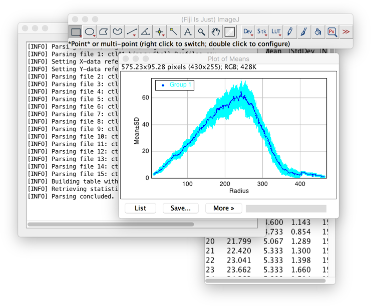
Analysis tool that 1) Merges individual Sholl profiles into a single table and 2) Obtains the average profile (with standard deviation) of a group of cells.
- File ▷ Open Samples ▷ ddaC Neuron
- Opens a sample image of a Drosophila class IV ddaC sensory neuron in which dendrites have been previously segmented (2D arbor). Use it to get acquainted with the plugin. Run Image ▷ Show Info... (shortcut: I ) to know more about this cell type.
- Help ▷ About Plugins ▷ About Sholl Analysis...
- Retrieves information about the plugin version and provides links to several resources including its source code repository and its API documentation. It is also accessible through the More » dropdown menu.
FAQ
General
- How do I cite Sholl Analysis?
-
The authoritative reference for Sholl Analysis is:
- Ferreira T, Blackman A, Oyrer J, Jayabal A, Chung A, Watt A, Sjöström J, van Meyel D. (2014), Neuronal morphometry directly from bitmap images, Nature Methods 11(10): 982–984.
- Schindelin J, Arganda-Carreras I, Frise E, Kaynig V, Longair M, Pietzsch T, Preibisch S, Rueden C, Saalfeld S, Schmid B, Tinevez JY, White DJ, Hartenstein V, Eliceiri K, Tomancak P, Cardona A. (2012) Fiji: an open-source platform for biological-image analysis, Nature Methods 9(7): 676-682.
- What is the difference between Sholl Analysis and an homonymous plugin released by the Ghosh laboratory in 2005?
- The original Sholl Analysis plugin by Tom Maddock (version 1.0) was released for ImageJ 1.35 and is now deprecated, unmaintained software that behaves erratically in newer versions of ImageJ. The current implementation of Sholl Analysis inherits Tom's initial 2D algorithm, but has numerous added features to enhance its utility. Note that throughout 2012 the plugin was temporarily called Advanced Sholl Analysis. You can follow the entire history of the plugin on GitHub.
- Why do I need to threshold the cell?
- Counting intersections is really a binary procedure: a shell either intercepts a branch or it doesn't. For this reason the image must be split in two phases: arbor and background.
- In version 1.0, it was not mandatory to adjust threshold values prior to analysis. Why is it now?
- Image segmentation has always been required. In its early implementations, the program dealt solely with binary images and used the intensity at the center of the analysis to decide how to segregate objects from background. This approach was very restringent: It assumed that the pixels representing the neuron would have the same (constant!) intensity that was not to be found in the remaining background. As the program became aware of grayscale images, this "feature" had to be removed because a single intensity can no longer be used to infer which parts of the image should be analyzed.
- My images do not look that great. How can I treat them prior to analysis?
- Have a look at Pre-processing.
- My bitmap profiles are different from the ones obtained from tracings of the same cells. Why?
- As mentioned several times, the quality of the analysis relies on how the arbor was segmented. If you are working with grayscale images you probably need to optimize your segmentation routines. On the other hand, if you already obtained binary images make sure you are interpreting them properly. You should also confirm that Ending radius does not intersect objects in the image canvas that extend beyond the analyzed arbor. As a rule of thumb, always refer to the Sholl mask to visually inspect which regions of the image have been measured.
- My version is not the latest after running Help▷ Update Fiji... Why?
- Please note that from version 3.4.6 onwards, updates are available through the Java-8 update site. If you have manually installed/modified Sholl_Analysis.jar (Development build?). Run the Updater, choose Advanced Mode then View locally modified files under View Options. Type "Sholl" in the Search field, selecting Sholl_Analysis.jar from the list of files. If the Details pane indicates an available update, click on Locally modified under Status/Action and choose Install/Update. The latest release version will be available once you press Apply changes. See Installation FAQs for more details.
- This documentation is not that useful. How long do I have to wait until it gets improved?
- Around 20 seconds. This is the time it will take you to create an account on this wiki. Once you have created one, you will be able to improve this page yourself.
Analysis
- The plugin complains about a wrong image type. Why?
- The plugin does not parse RGB images, but will process any grayscale image (8/16-bit), including multi-channel (composite) images. This is intentional: RGB images are inflexible and images of fluorescence-labeled cells are typically non-RGB images. As explained in the ImageJ User Guide, RGB images can be converted using Image ▷ Color ▷ Channels Tool... or Image ▷ Type commands.
- I cannot see the hemicircle/hemisphere option. Why?
- This option is only available if an orthogonal line has been created by holding ⇧ Shift when using the Straight Line Selection Tool. See the ImageJ User Guide for the full list of key modifiers that can be used while creating straight line ROIs.
- With 3D and 4D images, how do I set the Z-position and of the center?
- The Z-position (depth) of the center of analysis is the active Z-slice of the stack. With multichannel (composite) images, the active channel also defines the C-position. Both are reported in the Sholl Results table.
- I cannot see the option to save the results. Why?
- The image you are trying to analyze is not saved locally. Saving it to a local directory (e.g., your Desktop or Home folder) should re-enable it.
- Why so many parameters?
- The plugin is designed for the analysis of a wide diversity of arbors and it is not biased to any particular cell type. The only way to ensure this broad applicability is to give users full control over the mathematical techniques used by the plugin to analyze sampled data.
Results
- How can I save/edit the Sholl Results table?
- Select the table, then choose File▷ Save As…The filename extension can be specified using the More » Options... command (see the ImageJ User Guide for details). Single cells cannot be modified from within ImageJ, but custom extensions (e.g., .csv, .xls or .ods) will allow the table to be imported by other spreadsheet applications.
- Can I modify the way data is displayed?
- Mostly, using Analysis ▷ Sholl ▷ Metrics & Options (also listed in the More » Options... shortcut), including the number of decimal places reported by the Sholl Results table or the usage of scientific notation. To resize plots, use the More » dropdown menu in the Options dialog.
- What is the Sholl mask?
- The Sholl mask (see example of CA1 cell) is simply an illustration: a maximum intensity projection of the analyzed cell in which intersection counts are used as pixel intensities. As explained in Output Options, its LUT can be modified, and intensities calibrated using ImageJ default commands. As mentioned, it can also be used to visually inspect for segmentation artifacts.
- The 3D profile looks worse than the 2D profile of the Maximum Intensity Projection of the same cell. Why?
- An anisotropic voxel size will have a strong impact on step size. On the other hand, 2D and 3D images can be sampled differently depending on the options chosen. If Image▷ Properties… (⇧ Shift+P) reports the appropriate spatial calibration, make sure to read Multiple Samples and Noise Reduction before deciding which type of images to use.
- The program terminates without warnings. What am I doing wrong?
- The program will not terminate without throwing an error message. However, do note that some exiting messages are displayed in the often overlooked status bar of the main ImageJ window. This is intentional, as it minimizes the frequency of modal windows popping up for each failed operation.
Metrics and Curve Fitting
- Would it be possible to retrieve the Area Under the Curve (linear Sholl plot)?
- Sure. But it would hardly be relevant for data sampled at fixed intervals. The area under the curve (AUC, the area between the sampled curve and the horizontal axis, i.e., its definite integral) could be estimated using, e.g., the trapezoidal rule. However, because data is always sampled at equally spaced intervals, doing so would be the same as multiplying Mean inters. by the distance between Ending radius and Starting radius. Thus, effectively, AUC is redundant with Mean inters., that is already an integrated measurement of the sampled data. On the other hand, one could retrieve the AUC of the polynomial fit, but such property is already covered by Mean value.
- The shape of the polynomial changes at the edges of the profile. Why?
- Inflection points at starting/ending radius are usually associated with a poor fit and/or the fact that all the radii in which no intersections were counted are ignored. The latter is required to calculate the Sholl regression coefficient, as log(0) is undefined.
- None of the fitting options is suitable for my datasets. What should I do?
- Have a look at Complementary Tools.
Batch Processing
- The code that the Macro Recorder produced does not seem to work. What am I doing wrong?
- It is likely that frequent interactions with the dialog prompt(s) (from which the Recorder retrieves user-specified parameters) have "confused" ImageJ. While this process is usually flawless, it may happen that repeated triggering of GUI-specific commands that are not recordable (e.g., Cf. Segmentation or Import Other Data buttons) may lead to an incomplete recording. The solution is to repeat the recording, while minimizing such interactions.
Development
- I found a bug. How do I report it?
- Report it in the ImageJ Forum or file an issue on GitHub. Don't forget to include the steps needed to reproduce the problem. You may also want to check the release notes for the latest development version to see if the issue has meanwhile been addressed.
Release Notes and Pre-releases
Releases notes are available on Github. If you do not mind unstable software, development builds may be found here. Once new features mature and no major issues are found these development versions will be made available, as usual, through the Updater.
Related Resources
- Simple Neurite Tracer (SNT) The remarkable ImageJ framework for semi-automated of two- and three-dimensional tracing. SNT performs Sholl using the Sholl Analysis plugin. On the other hand, Sholl Analysis uses SNT to analyze tracings
- NeuronJ Another option for 2D reconstructions. NeuronJ features a friendly interface but is restricted to 2D images, is not capable of SWC export and is no longer under active development
- Neuroanatomy Resources in this wiki
- Neuroanatomy update site, distributing e.g., the Strahler_Analysis plugin
- BAR, Broadly Applicable Routines that complement Sholl Analysis
Publication
- Ferreira T, Blackman A, Oyrer J, Jayabal A, Chung A, Watt A, Sjöström J, van Meyel D. (2014), Neuronal morphometry directly from bitmap images, Nature Methods 11(10): 982–984
Citations
While in development (2005-2014), and prior to its publication, Sholl Analysis has been cited by several manuscripts. The manuscripts citing its 2014 publication can be retrieved using Scholar or PubMed. Below is a list of publications from authors that have made the developer aware how the program contributed to their research.
- Stanko JP, Easterling MR, Fenton SE. Application of Sholl analysis to quantify changes in growth and development in rat mammary gland whole mounts. Reprod Toxicol. 2015 Jul;54:129-35 PMID 25463529
- Kroner A, Greenhalgh AD, Zarruk JG, Passos Dos Santos R, Gaestel M, David S. TNF and increased intracellular iron alter macrophage polarization to a detrimental M1 phenotype in the injured spinal cord. Neuron. 2014 Sep 3;83(5):1098-116 PMID 25132469
References
- ↑ Ferreira TA, Iacono LL, Gross CT. Serotonin receptor 1A modulates actin dynamics and restricts dendritic growth in hippocampal neurons. Eur J Neurosci. 2010 Jul;32(1):18-26. PMID: 20561047
- ↑ Sholl DA. Dendritic organization in the neurons of the visual and motor cortices of the cat. J Anat. 1953 Oct;87(4):387-406. PMID: 13117757
- ↑ Brown KM, Barrionuevo G, Canty AJ, De Paola V, Hirsch JA, Jefferis GS, Lu J, Snippe M, Sugihara I, Ascoli GA. The DIADEM data sets: representative light microscopy images of neuronal morphology to advance automation of digital reconstructions. Neuroinformatics. 2011 Sep;9(2-3):143-57, PMID: 21249531
- ↑ 4.0 4.1 4.2 Ristanović D, Milosević NT, Stulić V. Application of modified Sholl analysis to neuronal dendritic arborization of the cat spinal cord. J Neurosci Methods. 2006 Dec 15;158(2):212-8. PMID: 16814868
- ↑ 5.0 5.1 Milosević NT, Ristanović D. The Sholl analysis of neuronal cell images: semi-log or log-log method? J Theor Biol. 2007 Mar 7;245(1):130-40 PMID: 17084415
- ↑ Schoenen J. The dendritic organization of the human spinal cord: the dorsal horn. Neuroscience. 1982;7(9):2057-87.PMID: 7145088
License
This program is free software; you can redistribute it and/or modify it under the terms of the GNU General Public License as published by the Free Software Foundation. This program is distributed in the hope that it will be useful, but WITHOUT ANY WARRANTY; without even the implied warranty of MERCHANTABILITY or FITNESS FOR A PARTICULAR PURPOSE. See the GNU General Public License for more details.
