Radial Symmetry
Download
The Radial Symmetry plugin can be downloaded from the update site. After that it will appear in the 'Plugins' menu under 'Radial Symmetry Localization'.
The source code is available on Github, please, also post feature requests & bug reports there.
Citation
Please note that the Radial Symmetry plugin available through Fiji, is based on a publication. If you use it successfully for your research please be so kind to cite our work:
<will be released soon>
Introduction
The Radial Symmetry Localization plugin enables users to find the smFISH spots with the super resolved accuracy. The software is designed for different types of imaging and is applicable to 2D/3D images together with the time-dimension.
The plugin is based on this paper. However, what makes the plugin really efficient is the usage of robust outlier removal. That makes the searching algorithm more stable when dealing with noisy images and helps to resolve the situations when there are multiple objects sitting next to each other.
Detailed Tutorial
Using the software package consists of the several steps. Please note that this is just a suggestion of how to use the package in the more-or-less standard case.
The basic setup looks as following:
- Find out how the z-scaling is different from the x-/y-scaling using the bead images.
- Run the program in the interactive mode to adjust the parameters for the particular dataset.
- Run the program in the manual mode (or even in the batch mode using ImageJ macro) to process the data.
Fixing Image Anisotropy
Since the resolution in z-axis might be much worse than the resolution in x- and y-axis we should perform the correction for that. To do that one will use the beads images acquired with the same microscope under the same conditions as the normal (data) images.
Open the image with the beads and navigate to the 'Plugins' > 'Radial Symmetry Localization' > 'Calculate Anisotropy Coefficient'.
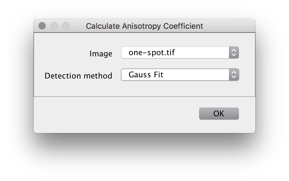
You will see the dialog window:
Choose the image for detection and set 'Gauss Fit' as a detection method. You can also try to use Radial Symmetry as a detection method but in this case Gauss fit gives better results.
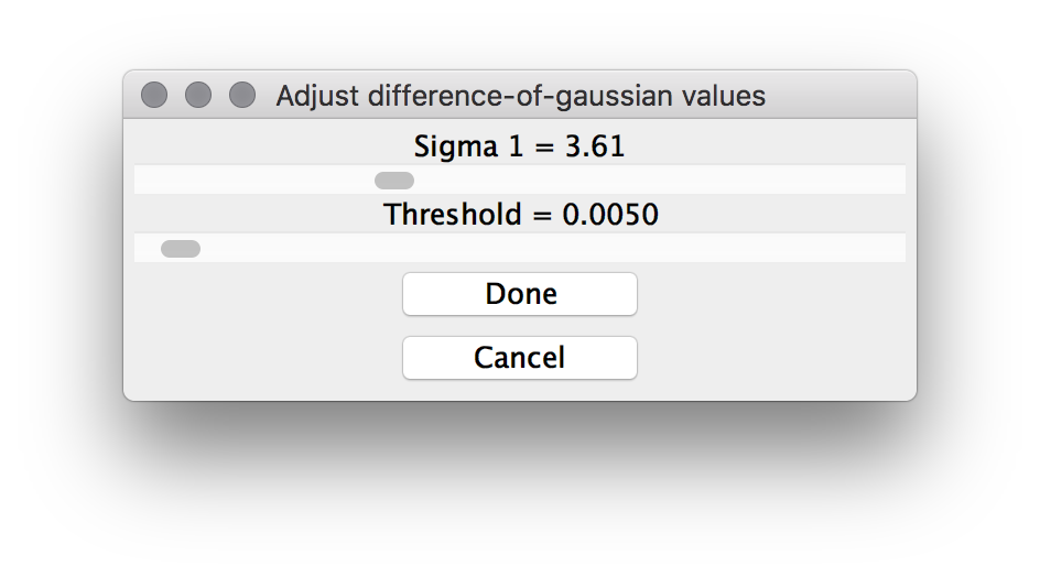
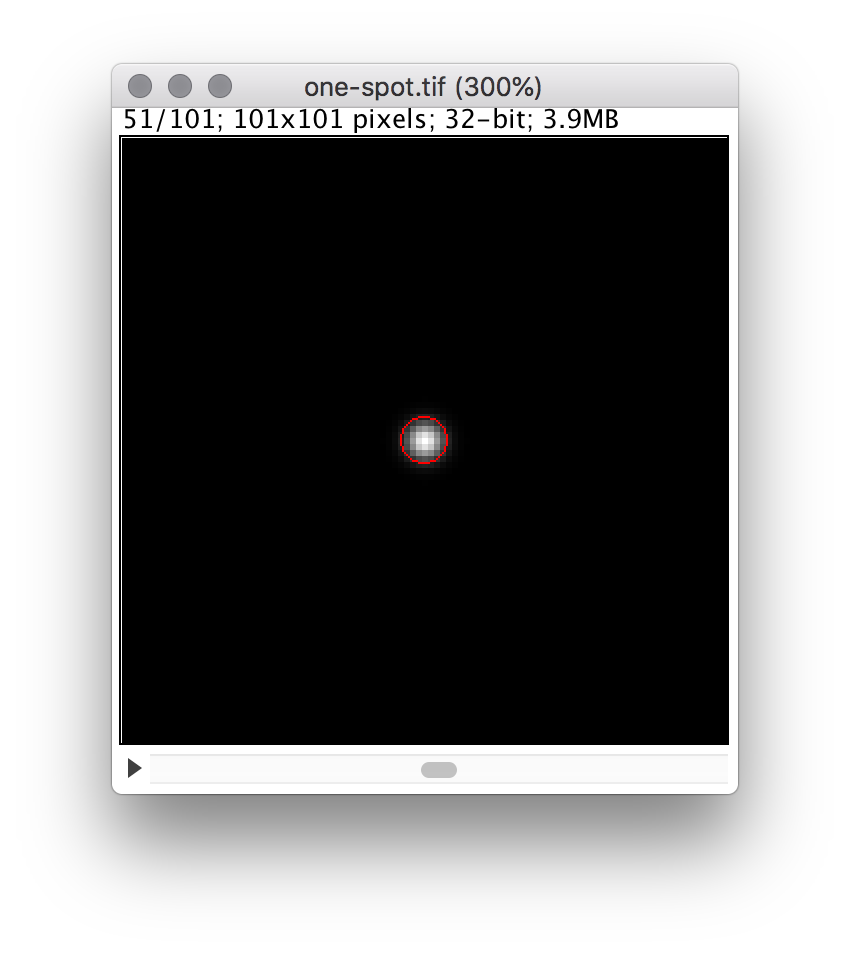
Once ok is pressed you will see 2 windows:
Adjust 'Sigma' and 'Threshold' values so that only beads are detected.
Once you are done – press Done button.
Depending on the number of beads the calculations might take some time. The program will calculate the corresponding anisotropy coefficient which basically shows how we should squeeze the objects in z-axis to make them look radially symmetric.
The corresponding anisotropy value will be shown in the Log window and it will be transferred to the next step automatically.
Important:
It is fine to skip this step if you do not have beads images. The plugin will be able to do decent job even with the default value of the anisotropy coefficient.
Localizing Spots
There are 2 different modes of processing images: interactive and manual. The Interactive mode is used to adjust the the parameters for further dataset processing. It also provides the visual feedback necessary to adjust the parameters for the automated processing on huge datasets.
Interactive mode:
Open the image and navigate to the 'Plugins' menu under 'Radial Symmetry Localization' > 'Radial Symmetry'.
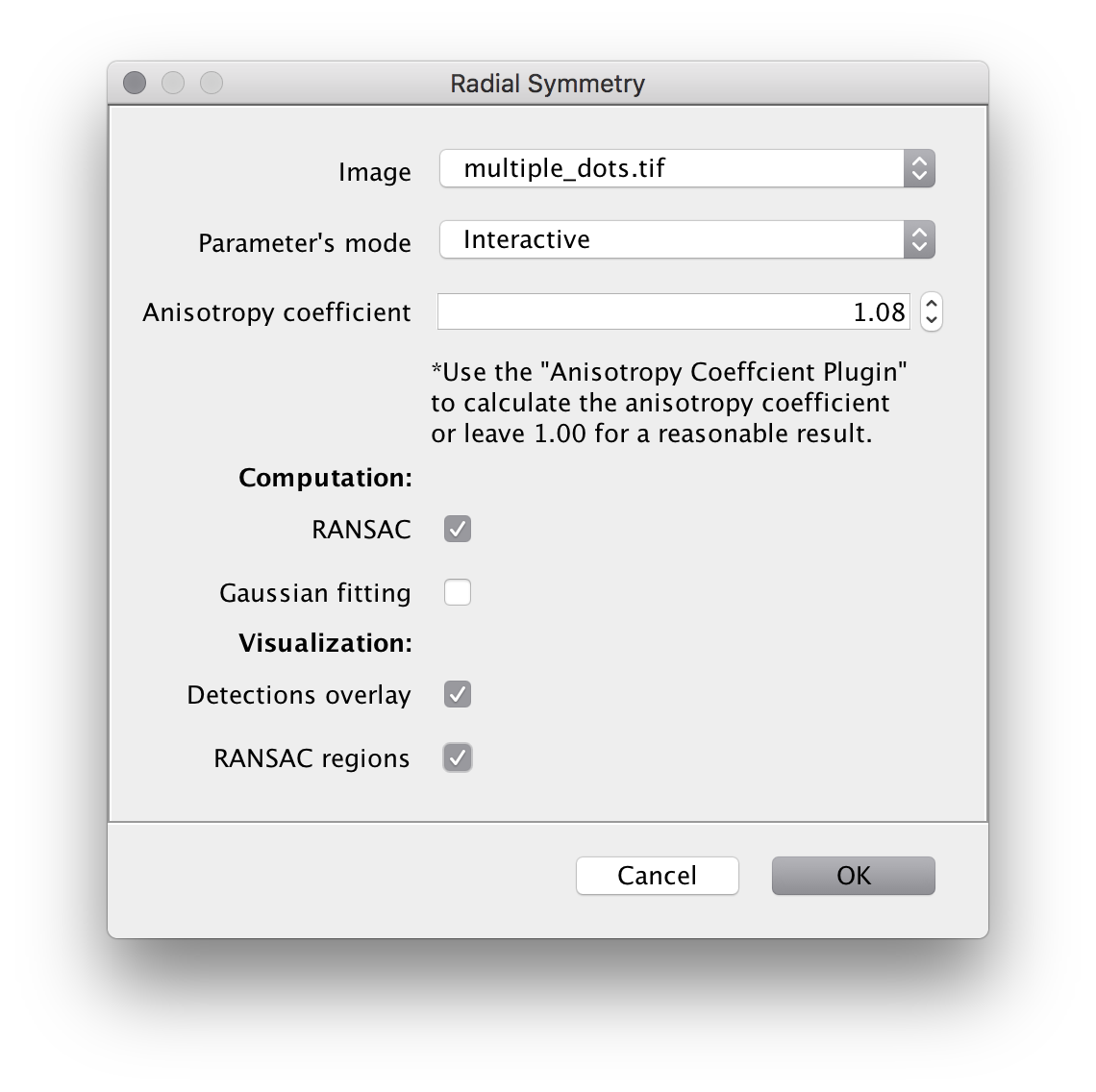
Window will pop up.
Ensure that the correct image is chosen.
There you have to setup some general parameters. Let us go though them quickly:
Since we do not know the best parameters for or dataset yet we set the 'Parameter's mode' to 'Interactive'.
Computation:
- 'RANSAC' defines if you want to use radial symmetry with or without the robust outlier removal.
- 'Gaussian fititting' defines if you want to perform the gaussian fitting algorithm on each of the spots that was detected. Ticking this option will give more precise intensity values but at the same time might significantly slow down the calculations. If this box is remained unticked the linear interpolation will be used to find the intensity values.
- 'Anistoropy coefficient' defines how much the z-resolution differs from the x/y-resolution. The parameter will be set automatically if you ran the 'Calculate Anisotropy Coefficient' plugin before-hand. In general, 1.0 gives the reasonable result. Warning: if you are working on 2D data you want see this checkbox.
Visualization:
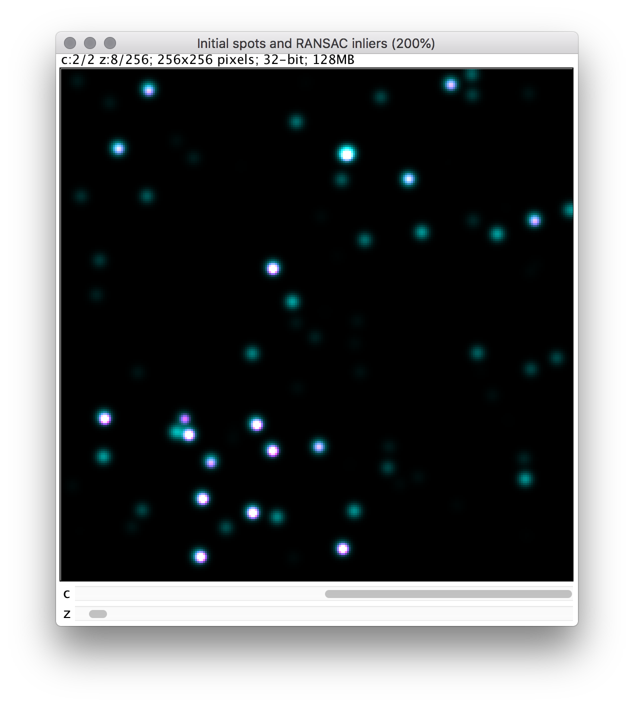
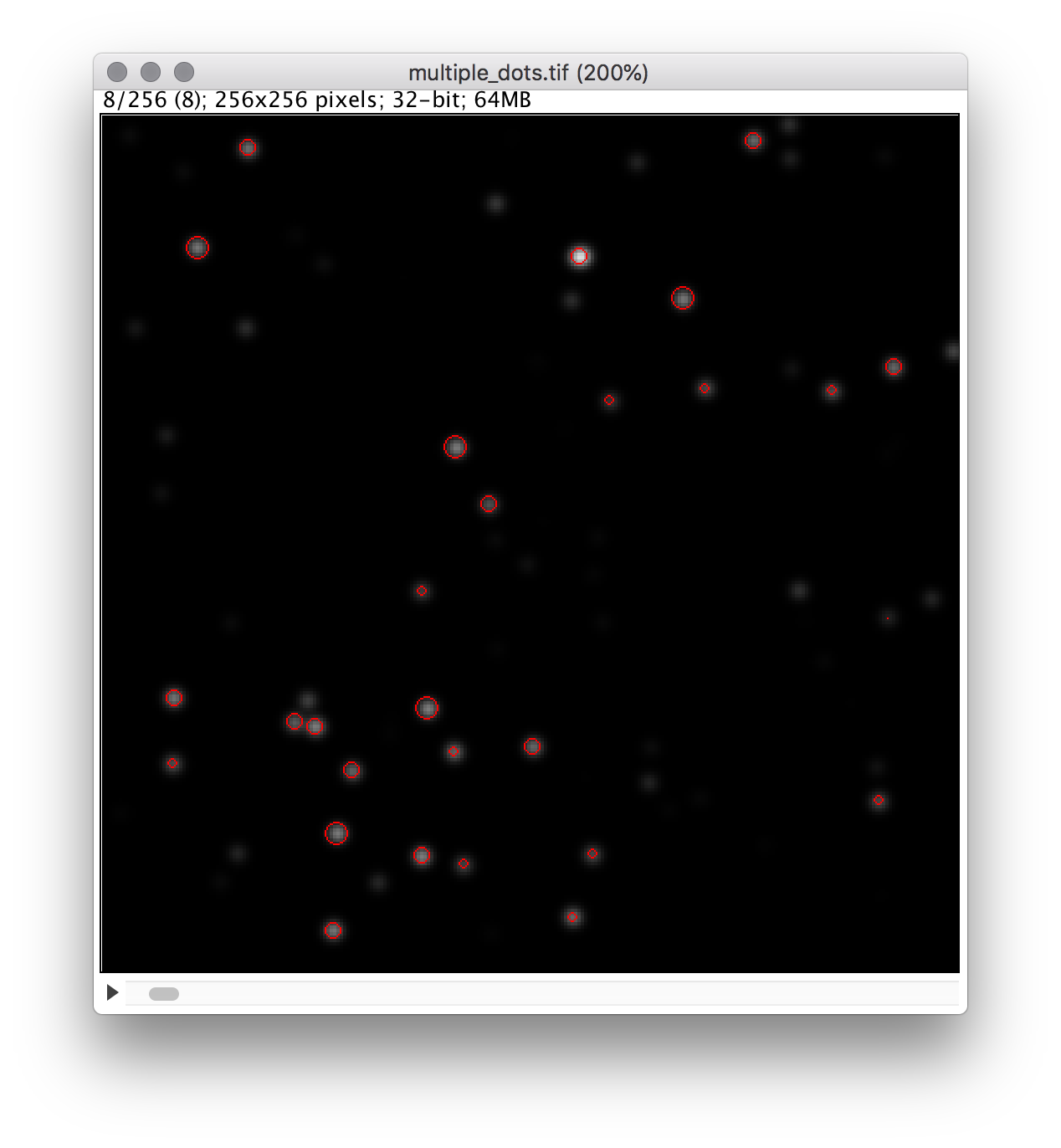
- 'RANSAC regions' shows overlay of the initial image with the regions that we used for the spots search.
- 'Detections overlay' shows the 3D overlay for the detected spots.
Once you are done with the settings press OK button.
After that you will see multiple windows.
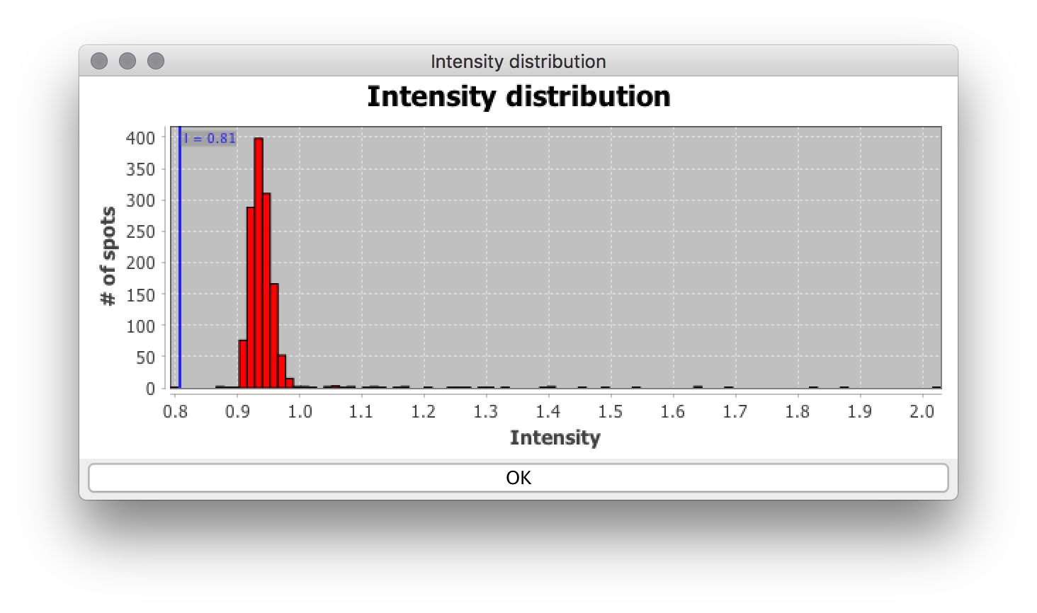
Difference of Gaussian window to adjust the corresponding parameters. This window is necessary to get rid of the false pre-detections. In general, we could skip this part but then the computations would take too much time. Adjust the parameters so that you do not have too many false detections. But also do not try to get rid of all of them – they will be discarded in the next computation step anyways.
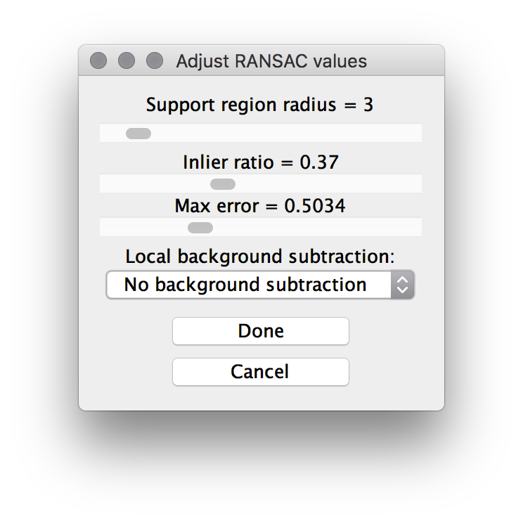
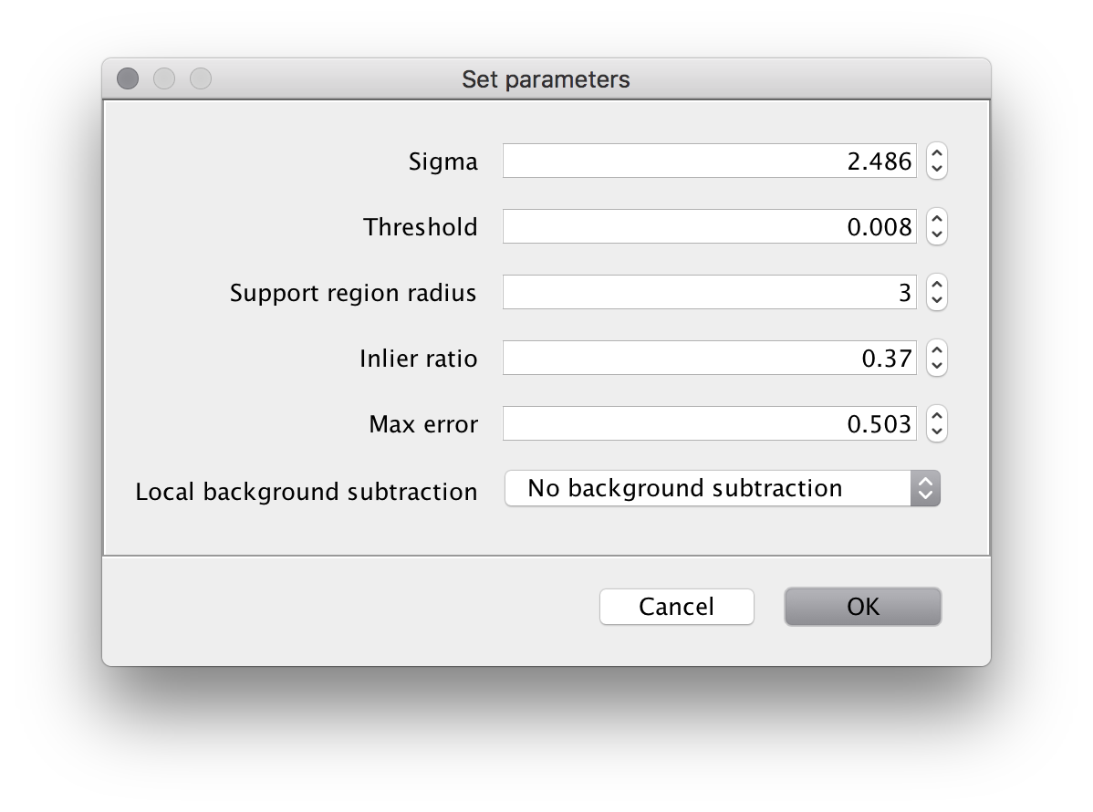
RANSAC window is the 'main' window of the whole plugin. Therefore, we will give a more detailed explanation for the parameters here.
'Support region radius' defines the radius of the spots we are looking for. You might want to play with this parameter. Sometimes it is useful to increase the radius and decrease the inlier ratio at the same time.
'Inlier ratio' defines the ratio of the pixels that should support the model. Simply speaking the ratio of pixels that should 'belong' to the current spot. Lower the number more detections false detections you will get.
'Max error'
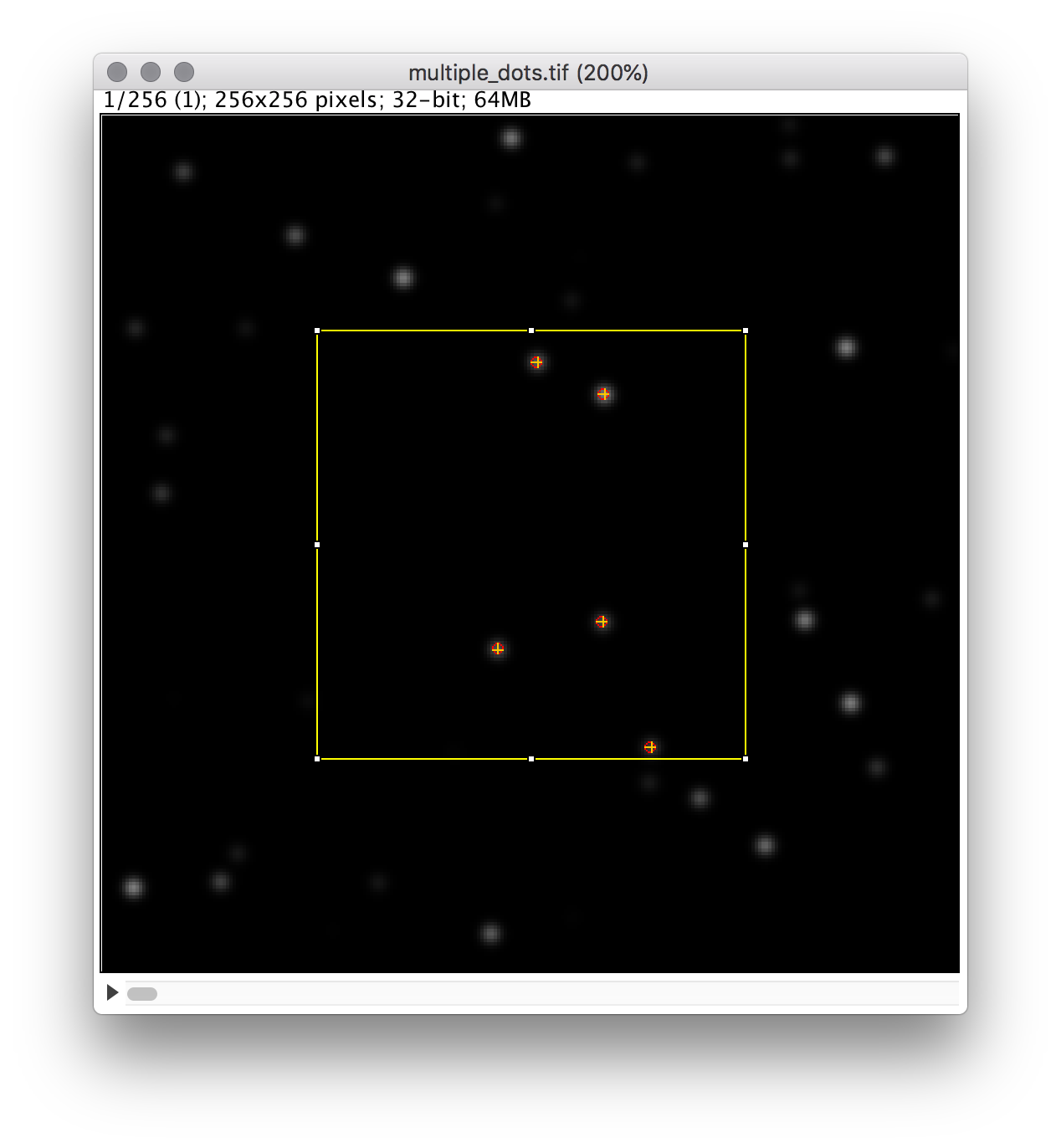
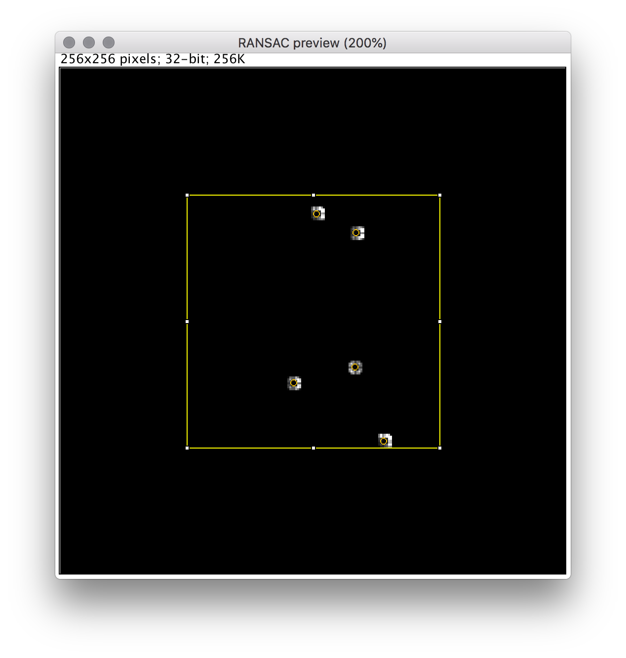
While moving the sliders you will see the updates in the two images.
One of them shows the pre-detections (red circles) and detections (orange crosses) in the provided region. Another one shows the pixels that were used by RANSAC and the error values at each of the used pixels.
Once the parameters are adjusted hit any of the 'Done' buttons and wait a bit while the computations are performed.
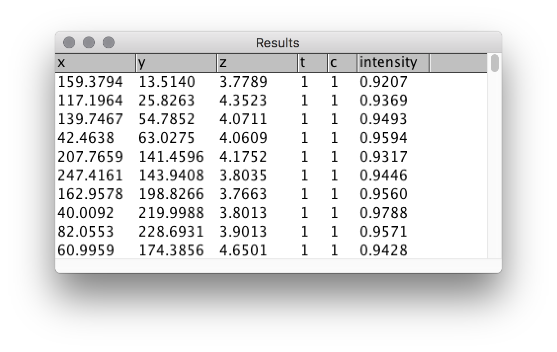
You will see the result table with the coordinates, time, channel and intensity values in the corresponding columns.
Besides that you will get 2 images: one of them showing the overlay of the initial image with the regions that we used for the spots search, another one showing the 3D overlay for the detected spots.
Manual mode:
In the manual mode you can skip all the hassle of the parameters adjustment and jump directly to the computations on the dataset.
After you choose 'Parameters's mode' manual in the 'Setup window' you will see all the parameters you have set already in the interactive mode. All you have to do now is to press 'OK' button and wait for the results.
