DiameterJ
| DiameterJ (ImageJ 1.48 or newer (including ImageJ 2.XX) and Fiji) | |
|---|---|
| Author | Nathan Hotaling |
| Maintainer | Nathan Hotaling |
| File | ImageJ 1.48a to 2.XXX DiameterJ v1.018
Fiji any version DiameterJ v1.018 |
| Source | Source Code |
| Initial release | February 2015 |
| Latest version | August 5th, 2016 |
| Development status | v X.003 (first version released publicly) |
| Category | Plugins Analysis |
DiameterJ[1] is a free, open source plugin created for ImageJ, ImageJ 2, and Fiji developed at the National Institute of Standards and Technology. DiameterJ is a validated nanofiber diameter characterization tool. DiameterJ is able to analyze an image and find the diameter of nanofibers or microfibers at every pixel along a fibers axis and produces a histogram of these diameters. Included with this histogram are summary statistics such as mean fiber diameter and most occurring fiber diameter (mode). DiameterJ also bundles OrientationJ[2] for a complete analysis of fiber orientation within an image as well as the "Analyze Particles" function built into ImageJ/Fiji to analyze pore space within scaffolds and produce summary statistics for pores.
Contents
Overview

- Image Segmentation into a binary image (black and white pixels only)
- Sixteen default segmentation algorithms have been included with DiameterJ in the "Segment SRM" and "Segment Mixed" plugins. However, these algorithms may not work for all SEM images.
- If the user is not happy with the results of the segmentation algorithms (i.e. the black and white images do not produce an accurate representation of the original image) then DiameterJ will still work with any binary image that has been segmented through some other means.
- Analysis of Segmented image
- All measures given by DiameterJ are in pixels by default
- DiameterJ has been validated with over 130 digital images created in silico and with scanning electron microscope images of reference wires with known diameters.
- - Fibers that are smaller than 10px or greater than 10% of the smallest dimension of the image produce 10% or greater error
- - For now DiameterJ only analyzes .tif, jpeg, png, .bmp, and .gif files
- - Fibers must be less than 512px in diameter to be analyzed
If you would like to cite DiameterJ in your work, citation information can be found here or use the below:
Citation/Reference Information
- Hotaling NA, Bharti K, Kriel H, Simon Jr. CG. DiameterJ: A validated open source nanofiber diameter measurement tool. Biomaterials 2015;61:327–38. doi:10.1016/j.biomaterials.2015.05.015.
http://www.sciencedirect.com/science/article/pii/S0142961215004652
Download Link
- For ImageJ 1.48 or newer: DiameterJ v. 1.018 for ImageJ
- For Fiji latest release: DiameterJ v. 1.018 for Fiji
How DiameterJ Works
The overall goal of the DiameterJ[1] algorithm was to be able to analyze an 8-bit SEM image of any resolution using a desktop computer in less than 60 seconds. For a block diagram and overview of how the DiameterJ algorithm analyzes fiber diameter and other scaffold properties see below.

Segmentation
SEM micrographs were first segmented using a variety of thresholding techniques available in ImageJ/Fiji. Both the Segment SRM and Segment Mixed plugins are automated inclusions of others segmentation algorithm work. Specifically, we have found that for SEM images of nanofibers the Statistical Region Merging algorithm[3] developed by Johannes Schindelin does a great job of blending fibers across their diameter and by depth to create great representations of the fibers when they are segmented. Additionally, we use more conventional segmentation algorithms developed by Otsu[4] , Huang[5], Kittler (min error)[6], Doyle (percentile) [7], or Zack (triangle)[8]
After segmentation all images had remaining noise and morphological features that were smoothed according to the protocols outlined by D'Amore[9] and by Gonzalez[10]. Briefly, successive rounds of noise removal (via ImageJ’s despeckle command) were performed until no change in the image was found. Erosion (through ImageJs erode command, and dilation (through ImageJs dilate command), and a final erosion (through ImageJs erode command), operations served to refine the image, highlighting fiber edges and eliminating isolated pixel areas. The described morphological procedures were performed to improve the precision of the centerline determinations as per the method developed by Lam et. al.[11].

Super Pixel Diameter
After image segmentation white pixels were summed for total fiber area in each image. Two different center-lines were then calculated for the image, one using an axial thinning algorithm developed by Zhang and Suen[12](Skeletonize command in ImageJ) and the other using a Voronoi tessellation[13] (Voronoi command in ImageJ). The axial thinning algorithm is very sensitive to changes in the fiber surface resulting in branches to areas that were not necessarily new fibers. The Voronoi algorithm essentially maximizes the distance between discrete black pixel clusters and thus is completely insensitive to fiber morphology. The length of each center-line was then averaged and the total area of fibers was divided by the average of the axially thinned and Voronoi center-line lengths. The two centerline lengths were averaged based on results from analyzing digital synthetic images and the finding that one method consistently overestimated fiber length while the other consistently underestimated fiber length.
The Super Pixel name was chosen because the fiber area, in pixels, was divided by the center-line lengths, in pixels; thus producing a unitless value that is equivalent to mean fiber diameter (fiber length x diameter = fiber area). This value is therefore a transformed pixel unit and is equivalent to the mean fiber diameter under the assumption that the fibers are just long rectangles when segmented into 2D shapes.
After its initial calculation the diameter calculation was then further refined via intersection correction. Intersection correction was done by taking the average length of the centerline and subtracting a radius value (obtained from first approximation of the diameter as determined without intersection correction) for each three-point intersection and a diameter value (obtained from first approximation) for each four-point intersection of the fibers. Intersections of each centerline were found using the algorithm developed by Arganda-Carreras et al.[14].
A new diameter was then calculated using the new corrected length and the total fiber area and this processes was looped until the diameter converged to 1/1000th of a pixel. Additionally, the number of intersections was also saved and the intersection density (ID) was calculated for a 100px x 100px (104) pixel area by dividing the total number of intersections by the total area (in pixels) of the image and multiplying by 104: 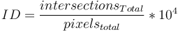 . The characteristic length (CL) of fibers was defined as mean length of fiber between intersections and was calculated by dividing the total centerline length by the number of intersections:
 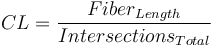 . The center-line length was calculated as the average of the axial thinning and Voronoi tessellation center-lines.
Fiber Diameter Histogram
Mesh Hole Analysis
Segmented pictures contain only black and white pixels; with black pixels representing background and white pixels representing fibers. Black pixels were analyzed using the Analyze Particles command in ImageJ. This algorithm essentially finds discrete clusters of black pixels, counts the number of pixels in each cluster and then reports their area. Pixel units were selected for particle analysis as well as a circularity from 0.00-1.00, the option to exclude clusters that touch the edge was also chosen. The subsequent particle analysis was then saved to later produce a mesh hole histogram, mean mesh hole area (produced by averaging all cluster areas), and percent mesh hole (produced by taking the total number of black pixels and dividing it by the total image resolution).
Fiber Orientation
Fiber orientation was determined using a well-established plug-in for ImageJ called OrientationJ[2]. To determine fiber orientation an axial thinning algorithm was used and then the centerline was enlarged by 2 pixels (using the Enlarge command in ImageJ) to ensure accurate measure of the line. Within OrientationJ a Fourier gradient was used with a gaussian window of 7 pixels. The subsequent frequency histogram of fiber orientation was then saved as an image. OrientationJ limits access to the raw data for this histogram; thus, if the user desires the raw data they must use the "OrientationJ Distribution" plugin. In the Fiji version of DiameterJ the Directionality[16] plugin, written by Jean-Yves Tinevez, can also be used to obtain the raw distribution data. This approach is considerably slower and less elegant (pop-up windows remain open) than OrientationJ but for now it is the only way to obtain the raw orientation data in batch.
How to Use DiameterJ
Learn DiameterJ Training Module
An in-depth training, called Learn DiameterJ, has been developed for users of DiameterJ. In total the training as been broken into 7 components:
- Initial Installation/Training/Use of DiameterJ
- Overview of how to install DiameterJ
- Training documents explaining general features of DiameterJ software/operation
- Detailed description of how to convert pixels to units for analysis
- Quiz to ensure understanding of concepts covered in the training documents
- Pre-Test
- For research purposes, this training is not required to learn how to use DiameterJ
- However, we'd appreciate it if you took the Pre-Test so that we can publish training results later
- Training 1 - Cropping and Segmenting
- How to crop images for use with DiameterJ
- How to segment images using DiameterJ
- Segmentation selection criteria for selecting the best segmentation from the options available
- Training 2 - Manual Segmentation
- This training covers how to efficiently manually correct image segmentations
- Training 3 - Assessment of Fiber Diameter
- Determining average fiber diameter,
- Identifican and use of histograms of the fiber diameter
- Multiple fiber diameters identification
- Selection criteria for when to accept a fiber analysis
- Training 4 - Other Metric Assessment
- How to use DiameterJ to assess other metrics of scaffolds
- Post-Test
- For research purposes, this training is not required to learn how to use DiameterJ
- However, we'd appreciate it if you took the Post-Test so that we can publish training results later
Please go to Learn DiameterJ to take the training!
DiameterJ Output
Summaries Folder | |
| "File Source Name"_Total Summary.csv | "File Source Name"_Total Summary.csv Continued |
|---|---|
|
|
Histograms Folder | |
| "File Source Name"_Pore Data.csv | "File Source Name"_Histogram.csv |
|
|
| "File Source Name"_Intersection Coordinates.txt | "File Source Name"_Radius Histogram.tif |
|
|
Diameter Analysis Images Folder | |
| "File Source Name"_Compare.png | "File Source Name"_Orientation.tif |
|
A montage image with four images in it
|
|
Limitations
- Due to mathematical limitations fibers that are smaller than 10px or greater than 10% of the smallest dimension of the image produce errors that are above 10% and thus deemed as too high for accurate measurement. This is because at small diameters (less than 10px) a single pixel error can cause 10% error in measurement. While with large fibers (greater than 10% of the smallest dimension of the image) low sampling and edge effects of fibers become a dominant factor in diameter distribution. This limitation can be overcome by altering your magnification when taking the image to make fibers smaller/larger as appropriate.
- Due to algorithmic reasons fibers that have a diameter larger than 512 px cannot be analyzed by DiameterJ. In general, this is not a concern if the researcher is taking images that do not violate the first limitation because an image would have to be over 5120 px on its smallest dimension for this limitation to affect them. However, with stitched images and with ultra high image resolutions (36MP or greater) this could prove to be a limiting factor. Work is underway to convert the Euclidean Distance Transform to a 16-bit algorithm that can analyze images with fibers that are 131,072 px or less in diameter.
- Images that have many fibers that entwine or that touch and run parallel to each other for long distances in an image can produce errant peaks in DiameterJ. This is usually due to segmentation of these images showing one larger fiber instead of many smaller fibers bundled. Additionally, images where partial fibers run along the edge of the image can cause DiameterJ to show fiber diameters that are smaller than the actual fiber. Thus, a "common sense" check on all images must be performed and while taking images the researcher must be careful to select areas where fibers do not overlap and run parallel considerably or run along the edge of the image.
- An integral part of analysis for DiameterJ is image segmentation. However, how an image is segmented into foreground or background can drastically alter the outputs produced by DiameterJ listed below:
- Normalized Orientation Index
- Mean Mesh Hole Size
- Percent Porocity
- Intersection Density
- Characteristic Fiber Length
- Fiber Orientation Histogram
- This is because the more fibers that are segmented out of an image the larger the pore size, the lower the intersection density and the higher the characteristic fiber length between intersections. Additionally, fiber orientation can be shifted because the orientation of underlying fibers can be different than the fibers that are closer to the top layer. Thus, while the algorithms analyzing these metrics are able to produce highly accurate results on calibration images; on real segmented images the analysis is entirely dependent on segmentation algorithm used. While, these algorithms were incorporated into DiameterJ to provide a reference way to calculate these values we caution that unless identical segmentation algorithms and image capture settings are used, results from these algorithms are not comparable between images.
- Fiber diameter is relatively invariant to segmentation because good image segmentation leads to having no partial fibers, only less fibers being included in the segmentation. Thus, while different segmentation algorithms may produce increased or decreased fiber sampling the measure of fiber diameters within each segmentation is accurate. Developing a segmentation algorithm that does not have this problem across any image is currently a topic of heavy research in the image analysis field.
- When analyzing the images with multiple distinct fiber diameters it has been found that DiameterJ under represented the prevalence of larger diameter fibers as compared to smaller fibers. This bias leads to weighted averages being inaccurate and for global averages of fiber diameters to be biased toward smaller fiber diameters. The bias is due to intersection correction/subtraction and the increased probability of larger fibers having more intersections due to their increased size. This limitation can be partially overcome by directional intersection correction of fiber intersection, which is currently under development. However, this limitation is inherent to all two-dimensional image analysis techniques and cannot be completely eliminated, making weighted averages of fiber diameter slightly inaccurate no matter what.
- Distinguishing between fiber diameters that are closer in diameter than 3 pixels often creates resolution difficulties for peak fitting and the prevalence of each fiber diameter can be skewed. This has to do with inherent limitations due to pixel binning of diagonal lines in Euclidean Distance Transforms. This limitation can be overcome by increasing magnification of your image so that fibers with different diameters have more than 3 pixels of difference between them.
Installation
If you installed imageJ before the end of 2013 you should uninstall your current version of ImageJ (DO NOT UPDATE) and reinstall ImageJ 1.48 or newer.
- Before uninstall be sure to copy all of your old plugins into a separate folder as these will be removed when you uninstall your old version of ImageJ.
- We recommend ImageJ over Fiji if you have no experience with either software because it is simpler to use.
| Download and install ImageJ 1.48 or newer or Fiji (any version) | ||
| Windows | OSX | Linux |
|---|---|---|
|
| |
FAQs
- Q: When running either segmentation algorithm an error occurs that says either "Unrecognized command: "Auto Threshold"" or "Unrecognized command: "Auto Threshold..""
- A: You have installed the wrong version of DiameterJ into your ImageJ/Fiji release. Fiji gives the "Auto Threshold.." error and it means you installed ImageJ's plugin into Fiji. ImageJ gives the "Auto Threshold" error and it means you've installed Fiji's software version into ImageJ0. Please download and install the correct version of DiameterJ for the piece of software you are using.
- Q: When I start ImageJ or Fiji for the first time after installing DiameterJ I get "Plugin configuration error: C:\... Duplicate command: "XXXX" (already in "YYYY")
- Where "..." is the directory where your plugin is located, "XXXX" is the name of the plugin and "YYYY" is the name of the directory where that plugin is already.
- A: You have duplicate plugins! Go to the file where you unzipped DiameterJ and its other plugins open the "DiameterJ", "OrientationJ", or "Analyze Skeleton 2D - 3D" folder" and delete the file named XXXX
- Where "..." is the directory where your plugin is located, "XXXX" is the name of the plugin and "YYYY" is the name of the directory where that plugin is already.
- Q: When I run DiameterJ an error occurs that says "Unrecognized Command: "Skeleton Intersections"" or "Unrecognized Command: "OrientationJ"" or "Unrecognized Command: "Analyze Skeleton (2D/3D)"" or "Unrecognized Command: "Statistical Region Merging""
- A: During installation one or more of the plugins that is needed for DiameterJ was missed. Please go back to the zip file that you downloaded for DiameterJ and copy all files into the plugins folder of ImageJ/Fiji
- Q: When I run DiameterJ an error occurs that says "Unrecognized Command: AAAA" where AAAA is any command not listed above.
- A: You are probably using a version of ImageJ that was updated to v. 1.48 or newer and did not create a fresh install of ImageJ. DiameterJ uses several plugins/scripts that ImageJ does not include in its updates, they ONLY include them in fresh installs. Thus you must uninstall ImageJ and reinstall a new version 1.48 or newer. Please remember save a copy of any plugins you added to ImageJ before uninstalling it, these will be lost during the uninstall process unless you save a copy in another location on your computer.
- Q: When I run DiameterJ an error appears in the log that says "Error there are no fibers in "BBBB".tif to analyze".
- A: The images that are in the folder that you have selected are not binary (black and white) images or the image is completely black. Please segment your image before trying to analyze it with DiameterJ and then move the segmented image into a separate folder with only black and white images in it.
- Q: No error occurs but when I ask the Segment XXX or DiameterJ to analyze a folder that I have images in, no output is produced by Segment XXX/DiameterJ.
- A: The image is probably not a .tif file. For now DiameterJ only analyzes .tif images. Please save your images as .tif files and then analyze with DiameterJ
- Q: DiameterJ keeps giving me an error on a file and won't continue on to the next file
- A: Unfortunately DiameterJ goes serially through files and isn't capable of skipping a file with an error. Simply remove the file that is giving the error from the folder you wish to analyze and rerun DiameterJ.
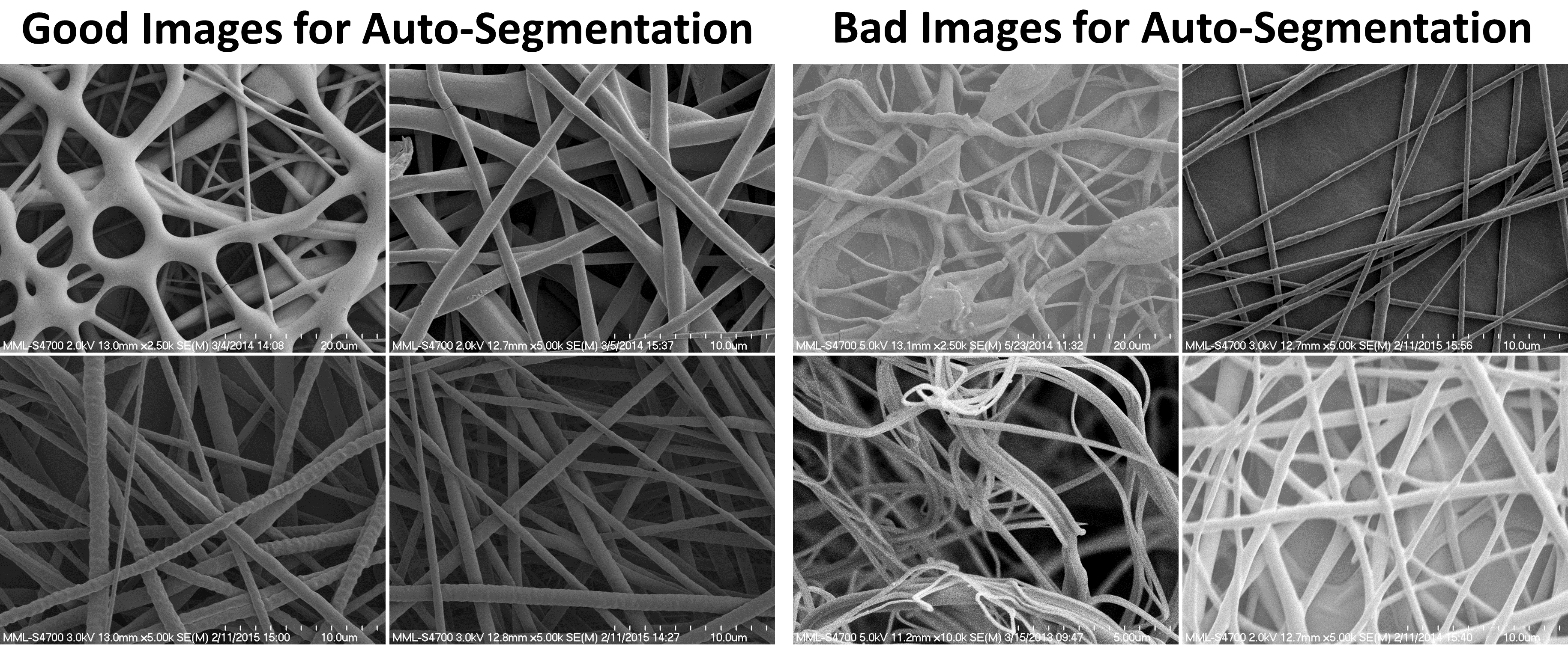
- Q: None of the images I am analyzing are segmenting well with your algorithms, why not?
- A: The algorithms included by default with DiameterJ rely heavily on uniformity of fiber color and/or a dark background. Below are four good examples and four examples that work poorly for image segmentation with the default algorithms. Keep in mind there are many more segmentation algorithms than I have included with DiameterJ in both Fiji and ImageJ. See the Complementary Tools or Image Segmentation sections of this work for a few of the options available.
- A: The algorithms included by default with DiameterJ rely heavily on uniformity of fiber color and/or a dark background. Below are four good examples and four examples that work poorly for image segmentation with the default algorithms. Keep in mind there are many more segmentation algorithms than I have included with DiameterJ in both Fiji and ImageJ. See the Complementary Tools or Image Segmentation sections of this work for a few of the options available.
- Q: When running either segmentation algorithm an error occurs that says either "Unrecognized command: "Auto Threshold"" or "Unrecognized command: "Auto Threshold..""

Complementary Tools
DiameterJ[1] works with several plugins of ImageJ/Fiji. First and foremost OrientationJ. Also, other great tools that we have incorporated are AnalyzeSkeleton function from Ignacio Arganda-Carreras, as well as Skeleton Intersections from Gabriel Landini's morphology plugin. We'd also like to give a big thank you to the Statistical Region Merging algorithm which makes our segmentations work a lot better. Speaking of which, we include a lot of segmentation algorithms that we aren't nearly talented enough to of developed ourselves. In particular those techniques outlined above in the Segmentation section of this article and can be found in the links below.
We'd also like to say that DiameterJ plays nicely with the output from any other segmentation algorithm that produces a binary image. Fiji has a ton of Segmentation algorithms that are great for different types of images. Additionally, many plugins have been created for use in ImageJ or Fiji: IJ Plugins Auto Threshold and Auto Local Threshold. If our defaults don't work then try any/all of these.
Finally, we'd like to encourage everyone to do peak fitting of the diameter histograms that DiameterJ produces. To do this any peak fitting tool can be used. A free resource for Windows is Fityk however, we don't recommend any software in particular.
Future Development
- Reducing bias of the Histogram intersection correction by directionally subtracting fiber intersections rather than blanket subtraction within a given intersection radius
- incorporation of Gaussian peak fitting algorithms within DiameterJ itself.
- Currently we are working on a native JAVA application on DiameterJ. This will not fundamentally change the function of DiameterJ however, it will make it faster, look cleaner, and should solve continuity issues
- 16-bit Euclidean distance transform calculator
- Enable DiameterJ to skip to the next file if an error occurs during analysis
Completed Goals
- Combine the three different releases of DiameterJ into a single release for all versions of ImageJ/Fiji
- Easier to use GUI (any GUI at all) with more options for what the outputs of DiameterJ are and what types of analysis it performs.
- Make DiameterJ compatible with images other than .tif files
Help is welcome in any/all of these improvements!
References
- ↑ 1.0 1.1 1.2 1.3 Hotaling NA, Bharti K, Kriel H, Simon Jr. CG. DiameterJ: A validated open source nanofiber diameter measurement tool. Biomaterials 2015;61:327–38. doi:10.1016/j.biomaterials.2015.05.015 http://www.sciencedirect.com/science/article/pii/S0142961215004652
- ↑ 2.0 2.1 R. Rezakhaniha, A. Agianniotis, J. T. C. Schrauwen, A. Griffa, D. Sage, C. V. C. Bouten, F. N. van de Vosse, M. Unser and N. Stergiopulos, Experimental investigation of collagen waviness and orientation in the arterial adventitia using confocal laser scanning microscopy, Biomechanics and modeling in mechanobiology, SpringerLink (DOI: 10.1007/s10237-011-0325-z)
- ↑ R. Nock, F. Nielsen (2004), "Statistical Region Merging", IEEE Trans. Pattern Anal. Mach. Intell. 26 (11): 1452-1458
- ↑ Otsu N. A threshold selection method from gray-level histograms. Automatica 1975;11:23–7.
- ↑ Huang L-K, Wang M-JJ. Image thresholding by minimizing the measures of fuzziness. Pattern Recognit 1995;28:41–51. doi:10.1016/0031-3203(94)E0043-K.
- ↑ Kittler J, Illingworth J. Minimum error thresholding. Pattern Recognit 1986;19:41–7. doi:10.1016/0031-3203(86)90030-0.
- ↑ Doyle, W (1962), "Operation useful for similarity-invariant pattern recognition", Journal of the Association for Computing Machinery 9: 259-267, doi:10.1145/321119.321123
- ↑ Zack GW, Rogers WE, Latt SA (1977), "Automatic measurement of sister chromatid exchange frequency", J. Histochem. Cytochem. 25 (7): 741–53, PMID 70454
- ↑ D’Amore A, Stella JA, Wagner WR, Sacks MS. Characterization of the complete fiber network topology of planar fibrous tissues and scaffolds. Biomaterials 2010;31:5345–54. doi:10.1016/j.biomaterials.2010.03.052.
- ↑ Gonzalez RC, Eddins SL. Digital Image Processing Using MATLAB, 2nd ed. 2nd edition. S.I.: Gatesmark Publishing; 2001.
- ↑ Lam L, Lee S-W, Suen CY. Thinning Methodologies-A Comprehensive Survey. IEEE Trans Pattern Anal Mach Intell 1992;14:869–85. doi:10.1109/34.161346.
- ↑ Zhang TY, Suen CY. A Fast Parallel Algorithm for Thinning Digital Patterns. Commun ACM 1984;27:236–9. doi:10.1145/357994.358023.
- ↑ Okabe A. Spatial Tessellations: Concepts and Applications of Voronoi Diagrams. 2 edition. Chichester ; New York: Wiley; 2000.
- ↑ Arganda-Carreras I, Fernández-González R, Muñoz-Barrutia A, Ortiz-De-Solorzano C. 3D reconstruction of histological sections: Application to mammary gland tissue. Microsc Res Tech 2010;73:1019–29. doi:10.1002/jemt.20829
- ↑ F. Leymarie, M. D. Levine, in: CVGIP Image Understanding, vol. 55 (1992), pp 84-94 http://dx.doi.org/10.1016/1049-9660(92)90008-Q
- ↑ Liu. Scale space approach to directional analysis of images. Appl. Opt. (1991) vol. 30 (11) pp. 1369-1373