Learn to set up and interpret multifractal analyses with FracLac.

Multifractal Analysis
    Using this Page:
  • Setting Options:
  • Interpreting Results: Click here
  • General Knowledge:

This page
explains the options and helps you interpret the results for a multifractal analysis.

Not the page you need? To learn how to use FracLac in general, try the basic tutorial; for a discussion of multifractals, go to the multifractal background page.

The page rather brazenly assumes you know all about using FracLac and have read the background section on multifractals. Cheeky, no? That said, you can click now on one of the three main sections (Options, Results, and Tips) to get on with your business, but, first and foremost, if you have not already, you really should learn about the key to doing a multifractal analysis - the Q.

Q is the easy part.

Q is part of the generalized dimension, D(Q), which is a key variable in multifractal analysis. Q is actually a range of exponents used to calculate and graph all of the variables in a multifractal analysis.

From the perspective of an innocent FracLac user, Q is just an arbitrary exponent—or, as we said, range of exponents—to specify.

The default Q–range is 0±10, incremented by 0.25 You set the maximum, minimum, and increment for the Q-range on the options panel. Experiment with Q settings to see how the multifractal spectra are affected for different images and ranges, but note that, in general, Q<−10 and Q>12 can cause calculation problems.

You may have already read about how to calculate the variables, including D(Q) in the multifractals page. Kudos if you can remember all the formulae!

Options
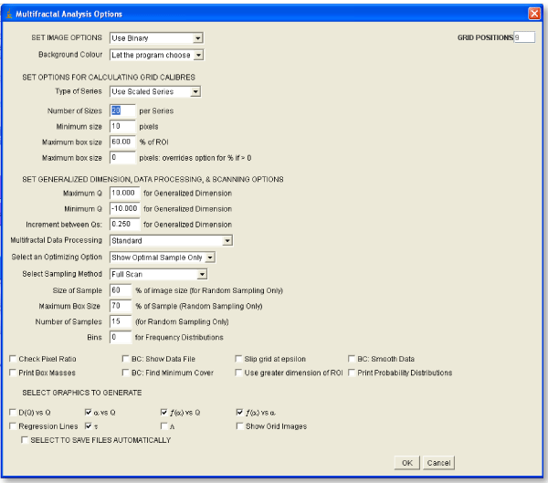
Now that you are primed for the practical part—analyzing—your next step is to click on the screen shot, on whichever options you need to learn about. You can also scroll down or jump to the list. The clickable screenshot shows the actual options panel that comes up for a multifractal scan; to find out how to bring up the panel, go here.

Options List

Save Files?

Select this option to automatically save files without viewing them on the screen (e.g., when doing batch jobs). See the saving tutorial for more.

Data Processing

Choose one of four choices from the drop-down box to determine what data processing to do when calculating multifractal variables and spectra. Note that this option affects how the multifractal variables are calculated, but not how the optional data file for standard box counting is affected.

  1. Standard.
    Select this option to process the pixel masses without filtering to calculate the multifractal spectra.

  2. Slope-corrected.
    Select this option to first filter the pixel masses by smoothing, which removes periods where box size does not affect the count, prior to calculating the multifractal spectra. This filter is especially useful for fixing sampling problems.

  3. Minimum cover.
    Select this option to first filter the pixel masses using a filter that selects the most efficient way of covering the foreground pixels prior to calculating the multifractal spectra. Be aware that this is a very limiting filter that can introduce problems for sampling in multifractal analysis (e.g., it does not do an exhaustive search for the most efficient covering; see optimizing in this regard).

  4. Slope-corrected Minimum Cover.
    Select this option to filter the pixel masses using a filter that smoothes (i.e., removes periods where box size does not affect count), then filter again to determine the most efficient covering prior to calculating the multifractal spectra. See the limitations noted above.

Number of Samples

Type a number for the number of random mass samples to take. This is ignored if the option for a random mass sample is not selected.

Maximum Grid (% of sample)

Type a number for the maximum grid calibre in a series, as a percentage of the sample size. This is ignored if the option for a random mass sample is not selected.

Size of sample(% of image size)

Type a number for the percentage of the total image size that you want to sample the image with. Note the total image size when you set this option so that your sample is neither too large nor too small. This is ignored if the option for a random mass sample is not selected.

Select Sampling method

Select "Full Scan" (recommended for most images) to scan the entire image once for each grid orientation or select "Random Mass" to randomly sample the image using the number of samples and sample size set in other options. (See Multifractal Sampling).

Increment between Qs for the Generalized Dimension and other multifractal variables

Type a number for the change from one value of Q to the next. See minimum Q and maximum Q.

Minimum Q for the Generalized Dimension and other multifractal variables

Type a number for the minimum to use for the arbitrary exponent, "Q" used to determine multifractal scaling. This is generally a negative number, but should be set taking into consideration the value to be used for the maximum Q - you may wish to bracket 0 by making the minimum -20 and the maximum +20, for instance.

Maximum Q for the Generalized Dimension and other multifractal variables

Type a number for the maximum to use for the arbitrary exponent, "Q" used to determine multifractal scaling. This is generally a positive number set in accordance with the minimum Q (e.g., you may wish to bracket 0 by making the minimum -20 and the maximum +20).

Bins for Frequency Distributions

See explanation in regular box counting options. See also print probability distributions.

Show Optimized Sample

Select an option from the drop-down menu.

  1. Show Optimal Sample Only
  2. Mark Optimal But Show All
  3. Don't Optimize

Select either the first or the second choice to filter the multifractal data using an optimizing algorithm; or select the third to show data and graphs for all grid orientations. Option 1, the first choice, is selected by default (see multifractal sampling).

If Option 1 or 2 is selected, the data are gathered and processed normally, but an optimal sampling orientation is selected from the final calculations by comparing the data from multiple grid orientations. The difference between Options 1 and 2 is only in what is shown; Option 1 discards all of the data and graphs except for the one grid orientation deemed optimal; Option 2 shows them all and indicates which was considered optimal.

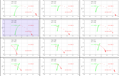
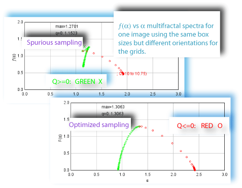
The number of grid orientations needs to be relatively high (e.g., more than 4 but dependent on the image) to use the optimizer effectively. The samples illustrated below, for instance, are ƒ(α) vs α spectra generated during one scan using 12 orientations for a Henon Map. The algorithm chose the highlighted instance. Note that it rejected samples where the graphs did not align, which reflect the major sampling issues inherent in box counting sampling that the optimizer is designed to address.

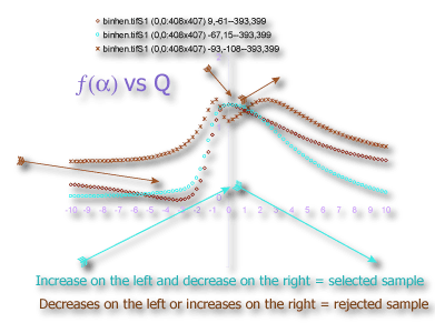
The optimal sample is selected by going down a hierarchical decision tree. The decision tree chooses the sample for which the maximum and the value at Q=0 for ƒ(α) were closest, then it compares in random order and selects on the basis of curving for ƒ(α) vs Q, as shown in the illustration.

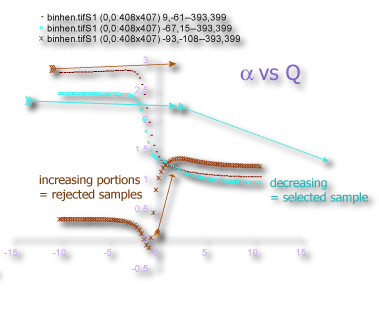
The next selection is made according to α vs Q decreasing, as illustrated in the figure, then, similarly, the generalized dimension, D(Q) vs Q decreasing and and dimensional ordering according to: theDcapacityDInformationDcorrelation

If the decision tree is traversed this far, the final steps use the sum of the values for positive Q and then the highest CV for D(Q).

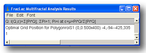
The optimum sample selected by the algorithm is graphed with the word "Optimized" in the graph's title, and the x,y coordinates of that grid orientation are printed on the graphic and recorded at the end of the results printed for the scan, in the results file, as illustrated below. If the option to show only the optimized sample is selected, then no other multifractal data are shown grahically and in the multifractal results file (box counting data will be shown for the other orientations in the data file, though.)Note that optimizing alone does not ensure that sampling is appropriate.

Λ

This option generates graphs of Λ or lacunarity data. (See a sample image here, read the glossary entry or click here to learn about lacunarity in general or here to learn about interpreting specific results). Note that the data from which lacunarity is calculated will be different in a multifractal scan compared to a regular box counting scan because the settings for grid sizes, sampling grid orientation, etc. are generally different.

τ

Select this option to generate
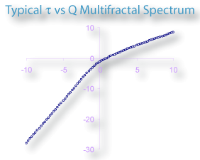
a graph of τ vs Q. The image shows a sample of the typical pattern for multifractals. See graphing multifractal spectra for more information. Two graphs are generated, reflecting two methods of calculating τ (Click for Calculations). Note that the optimizer will affect your results if also selected.

Regression

See explanation in regular box counting options.

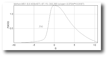
ƒ(α) vs α

Select this option to generate
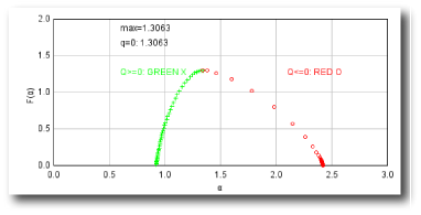
a graph of ƒ (α) vs α . The image shows a sample of the typical pattern for multifractals, with a green portion for values of Q≥0 and red for Q≤0. See graphing multifractal spectra for more information. (Calculations). Note that the optimizer will affect your results if also selected.

The maximum and value at Q=0 are listed on the graph. At Q=0, the generalized dimension is equal to the box counting dimension. See graphing multifractal spectra.

ƒ(α) vs Q

See graphing multifractal spectra

Select this option to generate
a graph of ƒ(α) vs Q. The image shows a sample of the typical pattern for multifractals. See graphing multifractal spectra for more information. (Click for Calculations). Note that the optimizer will affect your results if also selected.

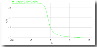
α(Q) vs Q

See graphing multifractal spectra

Select this option to generate
a graph of α(Q) vs Q. The image shows a sample of the typical pattern for multifractals. See graphing multifractal spectra for more information. (Click for Calculations). Note that the optimizer will affect your results if also selected.

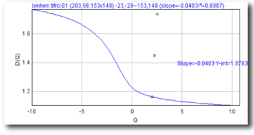
DQ vs Q

See graphing multifractal spectra

Select this option to generate
graphs of D(Q) vs Q. The image shows a sample of the typical pattern for multifractals. See graphing multifractal spectra for more information. Two graphs are generated when this option is selected, one graph bounded by the actual minimum and maximum D(Q) values (see image) the other by 0 and 3, so that multiple images can be readily compared. (Click for Calculations). Note that the optimizer will affect your results if also selected.

Slip Grid at ε

See explanation in regular box counting options.

Probability Distributions

Check this option to generate
a data file listing for each grid the frequencies and pixel masses in binned probability distributions at each ε (or boxsize). This is ignored if bins is less than l. Click the thumbnail to learn how to interpret the BPD file.

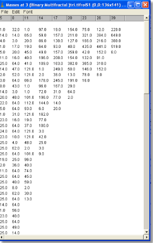
Print Box Masses

Writes a file for each grid location showing columns of the pixel mass labelled across the top of the file for each box size for each box laid on an image, as shown in the screenshot below. The file is named as "image name" "Slice" (X,Y: widthxheight)roi starting x,roi starting y--roi ending x, roi ending y.

Show data

Select this box to generate a box counting data file in addition to the Multifractal Results file. Note that the actual results of this file from a multifractal scan and a box counting scan may differ because of differences in sampling between the two types of analysis (e.g., grid orientation and the series).

BC: Find Minimum Cover

Select this option to apply a minimum cover filter to the DB in the data file for box counting; note that this option applies the filter ONLY to the data file and not to the multifractal spectra.

BC: Smooth Data

Select this option to apply a smoothing filter to the DB in the data file for box counting; note that this option applies the filter ONLY to the data file and not to the multifractal spectra.

Maximum box size pixels

See explanation in regular box counting options. See Tips also.

Use greater dimension of ROI

See explanation in regular box counting options. See Tips also.

Maximum box size % of ROI

See explanation in regular box counting options. See Tips also.

Minimum size

See explanation in regular box counting options. See Tips also.

Sizes per series (0 automatically calculates)

See explanation in regular box counting options. See Tips also.

Type of series

See explanation in regular box counting options. See Tips also for further information.

Show Grids

See explanation in regular box counting options.

Check Pixel Ratio

See explanation in regular box counting options.

Background Colour

See explanation in regular box counting options.

Number of Grid Positions

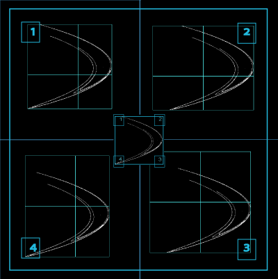
Set the number of sampling grid orientations to use. The sampling grid of the largest calibre for the first four orientations is oriented to rest respectively at each of the four corners of the bounding box, as shown in the image below. If the number is greater than 4, the rest of the grid positions are determined randomly based on the 4 corners. TROUBLESHOOTING: Click here if all of the origins are the same in your results file. If the number is less than 1, it is changed to 1. Multifractal sampling is discussed further in the background section. For a discussion of grid position in general, click here. To see the grids actually used, select "Show Grids".

Use Binary

See explanation in regular box counting options.

Results

Data Files

The results files and graphics returned from a multifractal analysis in FracLac depend on the settings in the options panel. The various data and graphics files from a multifractal analysis scan are listed below. Multifractal Spectra, Calculations, and sampling.

Graphics Files

Use the links below to help you interpret the various graphics. All of the graphics are generated by selecting them individually on the options panel. Click on the links to find out about them.The other graphics are explained in the links from the options panel, which you can also access here:

Results Files

  • For the Multifractal Results File, click on the column headings in the screen shot or use the links below:
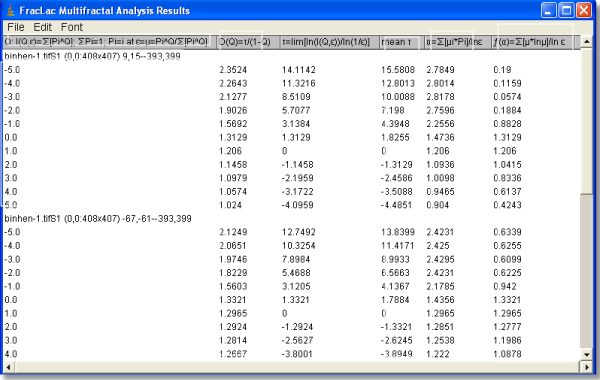
  • Calculations: The columns in the results file are calculated as follows:
    1. Q = The range of Qs specified in the options panel.
    2. Then, the rest of the calculations use the following results from the scan:
      N[ε] = the number of boxes from the box count at some ε
      m[i,ε] = mass at any box, i, at ε
      M[ε]=N[ε] i=1m[i,ε]
      P[i,ε] = m[i,ε]/M[ε]
      S[ε](Q)=N[ε]j=1(P[j,ε](Q))
      μ[i,ε](Q)= P[i,ε]/S[ε](Q)
    3. The Generalized Dimension
      D(Q)=τ(Q)/(Q-1)
    4. The τ column
      τ(Q) =(Q×α(Q))-ƒ(Q))
    5. The mean τ (Q) column = the slope of the regression line for ln τ[ε](Q) vs ln ε, where:
      τ[ε](Q) = N[ε]-1×N[ε] i=1[(m[i,ε]/M[ε])Q-1]
    6. α(Q) = the slope of the regression line for A[ε](Q) vs ln ε where
      A[ε](Q) =Ni=1 μ[i,ε](Q) × ln P[i,ε]
    7. ƒ (Q))= the slope of the regression line for F[ε](Q) vs ln ε where
      F[ε](Q) =Ni=1 μ[i,ε](Q) × ln μ[i,ε](Q)
    • Along with each set of 6 columns of data is a filename with numbers to identify the image, slice, roi coordinates and size, and grid coordinates and size. This information is changed and printed before each set. If the optimizer is selected, the set includes rows explaining the selection criteria and how the sample at the specified coordinates met those criteria.
    • See Multifractal Calculations

    Tips

    The defaults for FracLac's
    multifractal scan are set up for a Henon Map (Right click here to download the sample). This may not be an appropriate baseline for your images, however, and you may need to adjust settings accordingly. Following are some pointers that may help if you experience unusual results with multifractal scans, including some workarounds for known bugs.

    All Origins are the Same

    For perfectly square bounding boxes using exact multiples of the bounding box for the largest grid calibre, the first four origins will be identical. This is a bug owing to the way FracLac calculates the first 4 in multifractal scans. A temporary workaround is to select a number higher than 4 to find extra, random origins (e.g., select 8 to get 4 random origins in addition to four identical ones).

    Unusual Spectra

    Sampling is usually the problem when your spectra are not quite right. If the graph of D(Q) is not decreasing, or the red and green parts of the MF graph of ƒ(α) vs α do not meet in a continuous curve or appear to cross over as in the example, for instance, sampling may be inappropriate and may reflect a density distribution that attributes too much importance to very small probabilities that appear at some, but not all, grid positions. Negative Qs are most affected. This may simply be a matter of needing to find a better grid orientation, for which the solution is to increase the number of samples, and select to optimize and use a slope-correcting filter. Other potential causes and their fixes are listed below.
    Using the Optimizer with Invalid Calculations

    If you are using the optimizer, and it appears to incorrectly select such a sample over a better one, there may be calculation errors. This occurs if the values for ± Q are too high. This is a known bug (July 2007) that is being worked on. If it is happening, there will be non-numbers in the some of the results files, and you may see non-numbers (i.e., unintelligble symbols) for "Max=¦¯µ∅ ∑ Σ ¶" printed on the graph of ƒ (α), for instance. A workaround is to try setting the maximum and minimum to a smaller bracket around 0 (e.g., to 5 and -5 instead of 10 and -10, for example).

    Invalid Sampling Owing to Problems with Resolution and Grid Calibre

    If there are no invalid number errors, increasing the sampling orientations does not correct the problem, and selecting to optimize is also unsuccessful, the minimum resolvable box size may need special attention. To correct this, try changing (usually increasing) the minimum grid size in pixels to a value appropriate for your image. The problem may also be in the upper end of the series, in which case increasing the maximum size or changing the selection at Use Greater Dimension of Roi can help. In some cases, selecting a different series (e.g., switching from scaled series to "default") from the Type of Series box on the options panel will fix the problem. In addition, changing (usually decreasing) the number of box sizes using the Sizes per Series option on the panel may improves the result.

    Very Long Processing Time

    The number of box sizes can affect your results and processing time. To reduce processing time, it is often helpful to reduce the number of box sizes (e.g., 10 or less). You can select a custom series or a power series, for instance, in the series option on the panel. If you are doing a random mass sample, using less samples or decreasing the sample size may help.

    Problems with Random Mass Sampling

    If you get strange results with a random mass sample, you may need to adjust the maximum box size as a percent to 100%, adjust the number of box sizes up or down, and ensure the minimum grid size in pixels is high enough (e.g., >5 or 10).