Online Manual for the
MBF-ImageJ collection

11 t-Functions
11.1
Correcting
for bleaching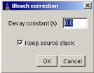
Often, during acquisition of a time-course, the fluorophore may bleach and the intensity of the image be reduced. This can make it harder to discern events at the end of the sequence. A stretch in contrast at time point 1 may not be adequate at time point 100. The process of bleaching and decrease in image intensity can be fitted with a mono-exponential decay, although it often follows a bi-exponential. A mono-exponential decay is described by the equation:
Corrected intensity = (Intensity at time t) ÷ exp-k×t k = decay constant
If you know the decay constant (k), you can use the “Plugins/Stacks - T-functions/Bleach Correction ” plugin. Run the plugin and enter the decay constant. It may be worth performing a background subtraction prior to running the plugin. Note that the plugin is expecting the k value to be “per-slice” rather than per-second, per-minute etc.
|
|
|
|
|
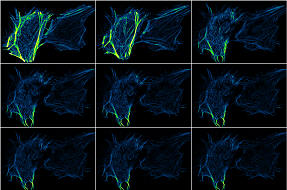
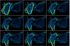
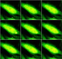
RAW
time course |
|
Bleach corrected time course |
The k value can be calculated in ImageJ by:
1. Make sure the “Edit/Options/Plot profile options” setting “Do not save X-values” is off.
2. Select a region of the cell or the whole image and plot the decay using the menu command “Image/Stack/Plot Z-axis profile”
3. Click the Copy button of the plot window.
4. Open the curve fitting dialog: “Analyze/Tools/Curve fitting”.
5. Delete the default data and paste in your copied data.
6. Select “Exponential” from the option list and click the “Fit” button.
7. In the Log window, scroll down to find the value labelled as “-b”, this is your k value.
Since bleaching is often not mono-exponential, quantification of fluorescence intensities after bleach correction is not possible. This plugin should really only be used to enhance time-course movies for presentation rather than quantification.
 Another
way to compensate for bleaching is to use the menu item “Process/Enhance
Contrast”. This method is quicker to implement than the proper bleach
correction above and can be useful for correcting for fluorophore bleaching
during a movie if the intensity of the fluorophore is changing only
because of bleaching. Check the “Process Entire Stack” option and the
plugin will scan through the stack applying Brightness and the contrast
adjustment selected on each slice based on each slice’s histogram (see section
7.2). The intensity values are adjusted so that quantitative
intensity measurements are no longer possible.
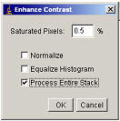
Another
way to compensate for bleaching is to use the menu item “Process/Enhance
Contrast”. This method is quicker to implement than the proper bleach
correction above and can be useful for correcting for fluorophore bleaching
during a movie if the intensity of the fluorophore is changing only
because of bleaching. Check the “Process Entire Stack” option and the
plugin will scan through the stack applying Brightness and the contrast
adjustment selected on each slice based on each slice’s histogram (see section
7.2). The intensity values are adjusted so that quantitative
intensity measurements are no longer possible.
Again, use this function to enhance movies for presentation, not quantification.
11.2 F÷F0
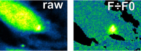
There are several drawbacks with the use of single wavelength fluorescent probes; some include uneven fluorescence intensity (F) due to cell thickness and cell to cell variation in loading. These can be largely corrected for by normalising fluorescence against resting fluorescence i.e. F0. This does not correct for bleaching and dye loss during the experiment.
First ensure the image is properly background corrected (7.5 Background correction).
11. Generate an “F0” image by averaging the first few frames of the stack. This can be done with the “Image/Stacks/Z-project”§ menu item, using the “Average” drop-down box option. Select “Start slice” as 1 and “Stop Slice” as 5-10 depending on how many frames you wish to average. Rename the new z-projected image (“Image/Rename”) “Fzero”.
2. Open the “Image Calculator Plus” via “Process/Image Calculator”.
3. Image 1 = Original stack
4. Image 2 = image “Fzero”
5. Operation = “Divide”
6. Select “32-bit Result” and “Create New Window”
7. Rename this result window (“Image/Rename”) FdivF0.
8. The maximum and minimum intensity in the stack can be determined with the “Analyze/Tools/Stack Histogram ” plugin.
9. Using the Brightness and Contrast (See section 4.1) dialog set the maximum and minimum to these values.
10. Convert the 32-bit stack to 8-bit (“Image/Type/8-bit”).
11. The Images in FdivF0 will probably have a noisy background between the cells and need to be cleaned up. Using your original stack, create a mask of the cells. This is done by first thresholding the original; stack (“Image/Adjust/Threshold”). Hit the Auto button and then adjust the sliders until cells are all highlighted red. Then click “Apply”. Check the tick box: “black foreground, white background”. You should now have a white and black image with your cells black and background white. If you have white cells and black background, invert the image with “Edit/Invert”.
12. Using the Image calculator “Process/Image calculator” to subtract this black and white stack from your FdivF0 stack.
13. Pseudocolour to taste.
This process could relatively easily be automated via a plugin or macro. However, due to multiple user-defined steps (i.e. how many frames for the Z-projection, the thresholding of the original stack for the mask, whether it’s better to correct for bleaching before thresholding the stack) I have not done so.
Much of this is automated in the plugin "Plugins/Stacks - T-functions/F divided by F0".
11.3 Delta-F
|
|
|
|
|
RAW |
|
Delta-F Up |
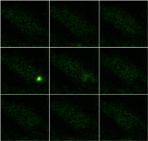
Rapid frame-to-frame changes in intensity (e.g. calcium “puffs” or TMRE “depolarisations”) can best be illustrated by performing subtracting each frame from the previous/next.
“Plugins/ Stacks - Tfunctions/Delta F up ”
For increases in intensity (e.g. a calcium “puff”) the calculation is [Frame(n+1)-Framen].
“Plugins/ Stacks - T-functions/Delta F down ”
For drops in intensity (e.g. TMRE plus irradiation induced mitochondrial depolarisations) the calculation is [Framen - Frame(n+1)].
11.4 Surface plotting
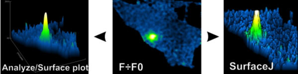

Surface plots can be generated in two ways: via the menu command “Analyze/Surface plot” or via the plugin “Plugins/VolumeJ/SurfaceJ ”. These functions will surface-plot movies as well as single frame images. Ensure the features you’re interested in are “Contrast stretched” optimally. This can be done using a “Max intensity projection” on the stack. Getting the max and min pixel intensities and applying these to the stack. Remember, do not perform intensity analysis on images that have had their contrast stretched.
11.4.1 “Analyze/Surface plot” settings
When this function is selected, a dialog will appear. Try the settings below first and play with them to optimise the surface plot. The LUT of the final surface plot is taken from the LUT of the image.
11.4.2 SurfaceJ settings
You can surface plot either a single frame or a movie. Surface rendering is a slow process so it is best to pick a frame from the movie that shows the features you’re trying to demonstrate. Duplicate this (Ctrl+D) and use it as a test image to get the best settings for surface plotting your movie.
Select the image to be rendered with the “Source image(s)” drop down box.
The options with three text-entry boxes along side represent x, y and z values.
“Rotate(°):” value of -20 in the first (x-axis) box gives a good 3D effect. Play with this.
“Scale”. Set to 0.5 speeds things along also when adjusting the settings and set to 2 or more for the final surface plotting.
“Aspect /:” Surface plot is can be stretched in “height” by increasing the z-axis aspect (i.e. the third) box. Although 1 is usually OK if you’ve stretched the contrast properly. This will not affect the pseudocolour of the peaks which is determined by the pixel intensity.
“Index LUT”: by default the plot will have the “spectrum” LUT. Change this drop-down box to “Load custom” and you’ll be prompted to locate a desired LUT when you start the surface-plot
“Gaussian Smoothing” value of 2-4. This slows rendering down but gives smoother surface plot.
“Rendering surface plot”: starts surface plotting.
§ ImageJ assumes stacks to be z-series rather than t-series so many functions related to the third-dimension of an image stack are called “z-” something – e.g. “z-axis profile” is an “intensity vs time” plot.