Colocalization by Cross Correlation
| Colocalization by Cross Correlation (Fiji) | |
|---|---|
| Author | Andrew McCall |
| Maintainer | Andrew McCall |
| Source | on GitHub |
| Initial release | 2020 |
| Development status | active |
| Category | Category:Plugins, Category:Colocalization |
This plugin attempts to determine the average distance between non-randomly spatially associated particles, the standard deviation of that distance (which should also reflect the width of the PSF in the image for diffraction limited images), and a statistical measure of confidence of the association. It currently works on 2D/3D single-channel images, and requires a mask of all possible localizations for the signal in one of the images.
Installing the Plugin:
Available on the list of ImageJ updates sites. Requires Fiji.
How it works:
The plugin performs a cross-correlation in frequency space to create a correlation image. To remove non-specific correlations (from background, or high signal density), a correlation image generated from randomized images is then subtracted from the original correlation image. This occurs through cycles of:
1. Randomizing Image1 using the Costes randomization method and a mask of all theoretically possible localizations for the signal in Image1 (i.e. a mask of the cells, or the nuclei).
2. Calculating the cross-correlation of the randomized image with Image2, then averaging this over successive cycles.
After the subtraction of non-specific correlations, we generate a radial profile of this data and fit a gaussian curve to it, showing the correlation between the images at different offsets. We also generate a radial profile for the original correlation data before subtraction, as this is needed to establish a measure of confidence. The confidence is calculated as the area under the curve (AUC) of the subtracted correlation radial profile (in the range of mean ± 3×sigma) divided by the AUC of the original correlation radial profile (in same range) as a percentage. The confidence value, along with the mean and sigma of the gaussian fit are displayed in a log window. Higher values of confidence, closer to 100, indicate that two images likely have a true spatial correlation at the indicated distance.
Preparing images:
This plugin requires two single channel, single frame images (2D or 3D) to be analyzed, and an additional binary mask to define the randomization area (details for mask below). The two images should undergo appropriate background subtraction to lower the background pixel values to zero or near zero. Even low level background (pixel values of 10 to 20 on a 16 bit image) can lower the confidence level and result in false negatives. Additionally, the images (particularly 3D) need to be correctly scaled (Image>Properties), otherwise all axes will be assumed to have the same scale. The mask for the binary image should cover all of the theoretically possible localizations for the signals in the image that is to be randomized. Typically this will simply be a binary mask of the cell volume, however if you are analyzing nuclear proteins, this would be a mask of only the nuclei. Using an inappropriate mask will likely result in the detection of a strong correlation caused by these higher order repeating structures (e.g. you will find a correlation at distances averaging 10-15 microns, caused by the repeating structure of the cells).
Running the plugin:
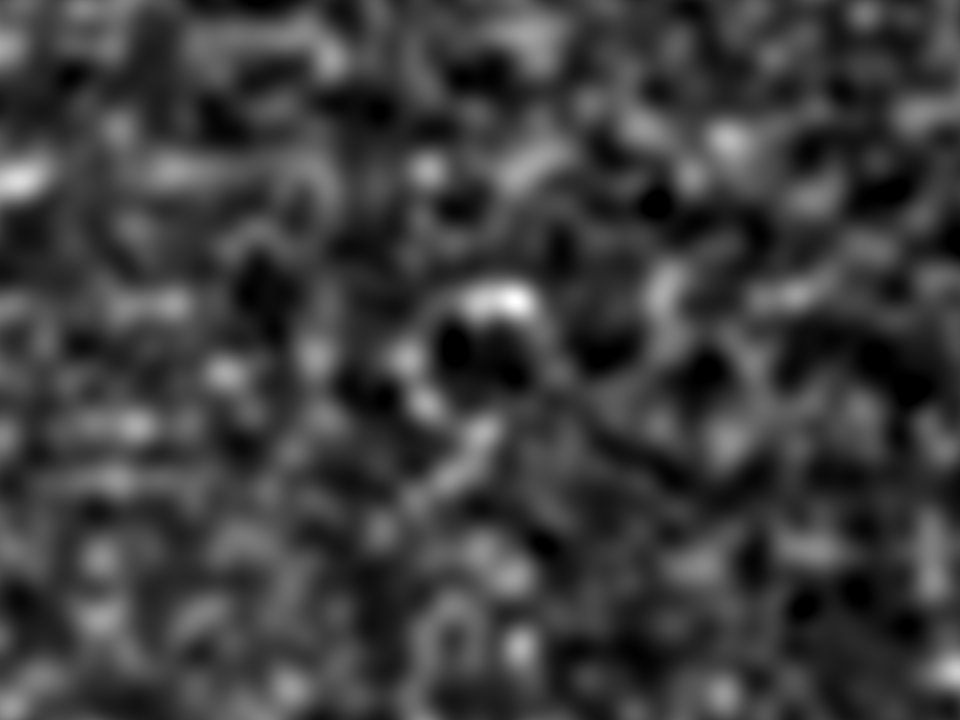
The plugin can be found in the plugins menu (near the bottom) and should be started with the images and mask already open. At the dialog menu, select the two images and the mask to be used, and enter the PSF width and height in pixel units. For the Costes’ randomization cycles count, you can typically input a low number (3-5), however if you have sparse signal within a large mask volume you will probably want to do more cycles. If the “Show intermediate data” box is checked, the plugin will open images showing the correlations (before and after subtraction of random associations), and a sample randomization image. This can be useful for understanding the function of the plugin, or for visualizing the direction of the correlation if your sample has a polarized axis.
Interpreting the results:
After the plugin has finished, two new windows will be open:
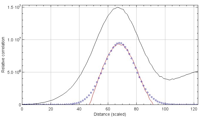
Correlation plot: A radial profile plot will be displayed, it contains the radial profile of the original correlation image (black line), the radial profile of the correlation after subtraction of random associations (red line), and a Gaussian curve fit to the subtracted profile (blue dots). The Y-axis is the result of the average correlation function at a given distance. While not arbitrary, it is most easily viewed as a measure of relative correlation. The range of the graph is set automatically to fit the Gaussian curve. If you wish to view all the data select More>Set Range to Fit all…
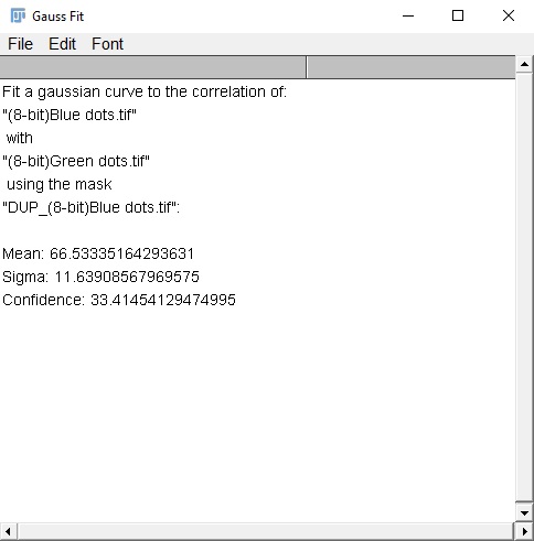
Gaussian fit analysis: This text window will contain (in scaled units), the mean distance for the discovered correlation, and the standard deviation of that correlation (sigma), as well as an estimation of confidence for this correlation (range 0-100). The confidence is determined by taking the area under the curve (AUC) of the subtracted correlation radial profile (in range of mean ± 3×sigma) divided by the AUC of the original correlation radial profile (in same range). Values closer to 100 indicate a strong likelihood of true correlation. Values near zero indicate low to no correlation between the two images. I currently estimate that values of ~20 or greater indicate some degree of correlation (within the range specified by the Gaussian curve), though this is with very limited data. Confidence values can be affected by many things, including image noise and background, an inappropriate randomization mask, and optical abberations. Performing a simple background subtraction can improve confidence scores signficantly.


