Coloc 2
| Coloc 2 | |
|---|---|
| Project | Fiji |
| URL | https://imagej.net/Coloc_2 |
| Source | on GitHub |
| License | GPLv3 |
| Release | 3.0.0 |
| Date | Wed May 03 13:28:06 CDT 2017 |
| Development status | Active |
| Support status | Active |
| Team | |
| Founders | Johannes Schindelin |
| Leads | Daniel James White, Tom Kazimiers |
| Developers | Ellen Dobson |
| Debuggers | Tom Kazimiers, Ellen Dobson |
| Reviewers | Daniel James White, Tom Kazimiers, Ellen Dobson |
| Support | Daniel James White, Ellen Dobson |
| Maintainers | Daniel James White, Curtis Rueden |
| Contributors | Johannes Schindelin, Jan Eglinger, Leonardo Guizzetti, Mark Hiner, Jean-Yves Tinevez |
Contents
- 1 What is Coloc 2
- 2 How to use Coloc 2
- 3 Pitfalls of the Manders and Costes methods
- 3.1 The auto threshold calculation method can fail if fed inappropriate information
- 3.2 Effect of noise on Pearson's and Manders' coefficients
- 3.3 Fluorescence emission bleed through looks like perfect colocalization
- 3.4 Regions of interest (ROIs)
- 3.5 Other pitfalls
- 3.6 Release Notes, Newly Added Features and Squashed Bugs
- 3.7 Ideas List
What is Coloc 2
Coloc 2 is Fiji's plugin for colocalization analysis. It implements and performs the pixel intensity correlation over space methods of Pearson, Manders, Costes, Li and more, for scatterplots, analysis, automatic thresholding and statistical significance testing.
Coloc 2 does NOT perform object based colocalization measurements, where objects are first segmented from the image, then their spatial relationships like overlap etc. are measured. This complementary approach is implemented in many ways elsewhere.
There are many nuances and pitfalls to colocalization analysis. As such, we strongly recommend you read the Colocalization Analysis section of the Cookbook before attempting to use Coloc 2!
How to use Coloc 2
- Read the original papers describing the analysis you are about to perform.
- Don't treat this tool as a black box - try to understand what the strengths and limitations are and what the results could mean.
- Open images to analyze.
- You need a 2 color channel image. If the image has more than 2 channels, identify the two you want to analyze with each other, then split the channels into separate images (Image- Color - Split Channels)
- Z stacks work fine. But time series will fail until that is fixed. For now, please split the time series into a numbered set of images and analyse those one by one. See https://github.com/fiji/Colocalisation_Analysis/issues/6
- You probably want to analyze only some region of interest (ROI), there are 2 ways to do that:
- Select a region of interest with one of the ImageJ selection tools, in one of the images.
- If the image is a z stack, then the ROI applies in all "slices" of the stack.
- You can have a third "binary mask" image, with the same x,y,z dimensions as the 2 images to be analyzed:
- where the mask image is white (255 pixel value for an 8 bit greyscale image) colocalization will be analyzed for those pixels only. Where it is black (zero pixel value), the pixels will be ignored: not included in the analysis.
- you can use a z stack as a 3D mask... it's up to you how you make that mask image, manually or by some automated method.
- Select a region of interest with one of the ImageJ selection tools, in one of the images.
- Launch the Coloc 2 plugin from the menu item: Analyze - Colocalization Analysis - Coloc 2
- or use the command finder: press L then start typing Coloc, then choose the plugin with the arrow keys and hit enter, or double mouse click it to launch the plugin.
- In the plugin's graphical user interface (GUI) choose the 2 images you want to analyze in the first 2 drop down lists.
- Select the images according to which you want to be channel 1 and which to be channel 2.
- In the third drop down list selection, select the image/channel you want to use that has the correct ROI or mask image
- remember: for the mask image - it must have the same xyz dimensions (number of pixels and slices) as the other 2 images.
- Choose which "Algorithms" are run and which statistics you wish to calculate, and if you want to save the "standardized" PDF result file, when the OK button is pressed.
- Numerical results and image names are dumped into the ImageJ Log window as comma separated values, so you can copy paste, or save the log window contents, to then import them into whatever statistical package or spreadsheet in which you wish to analyze the results.
- Turn the options on/off by clicking the selection button at the left of the Algorithm description
- Also choose the approximate size of the point spread function (PSF) in your images, as well as the number of iterations to run the Costes statistical significance test (We suggest a large number... the larger the number, the longer the analysis will take. Do, at the very very least, 10 iterations (100 would be better).)
- You should know approximately how big the PSF is (in pixels) in your images.
- If you don't, go back and read about: What is the PSF? Why is it important in colocalization analysis? (for instance: read the Costes paper )
- This size determines what size of image 'chunks' are shuffled in the randomization process. (PSF-sized image pieces make physical sense, as that's the size of the smallest features visible in the image.)
- Click OK to run the analysis.
- The results gui will open showing a table of numbers and one of several images
- the images can be chosen on the Dropdown list.
- You can see the 2 Li plots, a scatterplot or 2D histogram with regression line, and input images and Roi.
- the scatter plot uses fire colour look up table.
- the log checkbox allows display of images with or without log scaling, useful for eg. the scatterplot
- You will be asked if you want to save the results as a PDF file (if the "Show Save PDF dialog" button was checked. So tell it where to save the PDF. This is standard output format, so you can compare with your friends, same vs. same.
- Feel free to tell us what things you think should be included in this standardized PDF output file and how it should be formatted. HTML? XML? Plain text?
Pitfalls of the Manders and Costes methods
The auto threshold calculation method can fail if fed inappropriate information
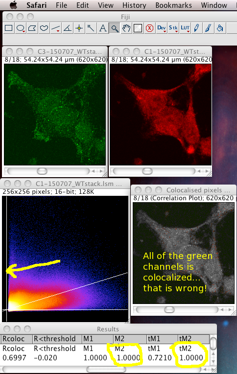
That means it does not like images with high zero offset, where no light detected still gives a large non zero pixel value. For instance, from a digital camera's zero offset/bias, or a confocal PMT's offset when incorrectly set. Also, a high, flat non specific background causes the same problem. These all add a constant number to the intensity values of each pixel, offsetting and obscuring the true proportionality relationship with the "concentration" of the fluorescent dye detected at each pixel. If pixels that contain no real (specific) signal have large intensity values, the algorithm, not knowing about the non zero intensity offset in all pixels, assumes the offset is real signal to be dealt with, and can reach a result for the thresholds where one or both of them is below the value of the lowest intensity value present in that colour channel of the image. This means that ALL of that channel's pixels are considered to be colocalised, then the Manders' Coefficients that you get will reflect that aberrant, unrealistic situation. In these cases, the background and/or offset should be carefully removed/subtracted before running the Coloc 2 or Colocalization Threshold plugin. The images below are an example of this situation, using the badly behaved data set: 150707_WTstack.lsm. Note that the values for M1 and tM1 are the same! This should not be the case. You can see the green channel threshold is wrongly set below the intensity where the image data intensities actually start.
Notice: the image contains large areas of background, with similar low values of pixel intensities in both channels. This means there is strong correlation in the background areas, which interferes with the interesting biological correlation in the high signal areas where the biology is located. This means it is important to set a biologically relevant region of interest (ROI) and not analyse the whole image. We must avoid analyzing the highly correlated, but uninteresting, background areas. See the section below...
Effect of noise on Pearson's and Manders' coefficients
In the case of perfect colocalization, where the intensities of the 2 channels are always perfectly correlated: Low red with low green, and high green with high red, the scatterplot would have all the data points falling on a straight diagonal line, since the green intensity would always be in proportion to the red! However, that is the ideal case and real biological data is noisy! Noise (be it from the dyes not staining every single molecule, or from statistical photon shot noise from recording the signal from too few photons, or from other electronics noise sources) will cause the pixel intensities to deviate from the perfect/true case, to be lower or higher than they really are on average. This causes scatter in the distribution of the data points in the scatterplot, perpendicular to the line of regression fit. So you can see the noise by looking at how spread or tight the scatterplot points are from the linear regression line. Also, since Manders' coefficients are measuring correlation, and noise lowers the similarity of two identical signals, noise lowers the Manders' coefficients to less than they should be for an image with very low noise. The same is true for Pearson's correlation. So for the same object under the microscope, noisier images will appear to give less colocalization than a clean, low noise, image. That means you can't compare different images with different signal:noise levels, unless you have some way of estimating the noise and correcting for it.
Background and digital offset should be subtracted (this doesn't affect Pearson's but does affect other measurements), and noise should be filtered out, suppressed or best avoided by collecting as many photons as possible. Deconvolution is a great way to restore images to give a better estimate of the real fluorophore spatial distribution by suppressing noise and removing the offset or background, while improving contrast and dynamic range by equalizing the spatial frequency response up to the objective lens resolution limit. Confocal images should also be deconvolved, not only widefield images, especially in the case of low signal and high noise.
Fluorescence emission bleed through looks like perfect colocalization
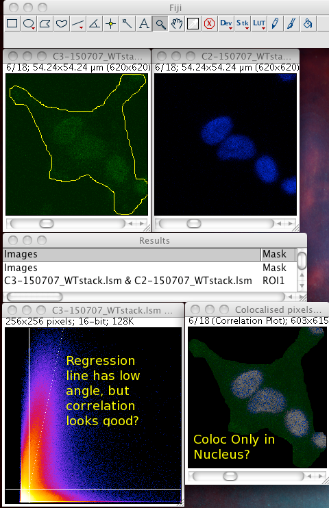
As is often true for DAPI nuclear stain and GFP dye pairs, when images are captured at the same time, with both dyes being excited and detected simultaneously, fluorescence emission bleed through gives misleading results, as the signal from the DAPI also appears in the GFP detection channel! Where there is more DAPI, there is also more signal in the GFP channel. This looks like really good colocalization, but of course it is totally false! It is a problem with the imaging systems not being set up correctly or not used correctly. This can also happen with many other dye combinations, if they have overlapping emission spectra. Always check your spectra. You can do that here: Invitrogen Fluorescent Dye Spectra Viewer. To be safe, check your emission filter sets don't allow in the wrong signal, and do "sequential imaging", so you only excite and image one dye at a time.
Regions of interest (ROIs)
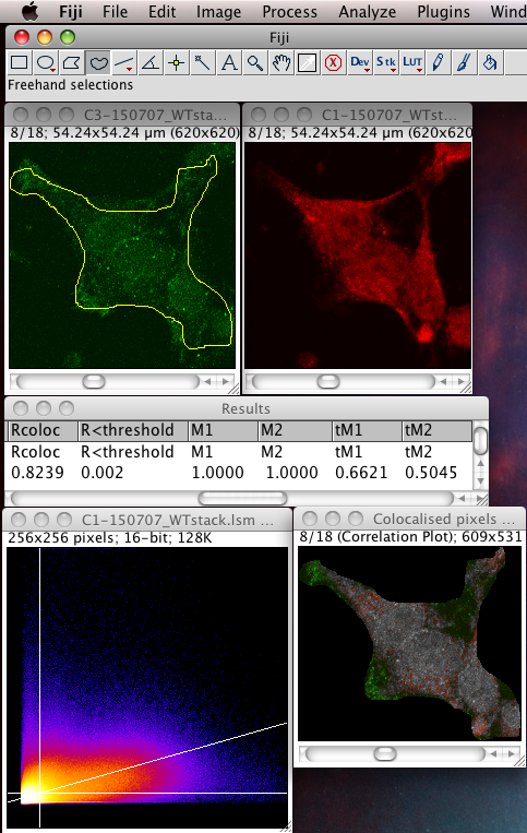
Whether or not to consider zero - zero pixels as part of the interesting data for the algorithms to deal with. If you think about it, in a fluorescence image there is typically quite a large area which is black in both channels. For instance where there is space between cells, or just no signal in either channel since that area is not part of an interesting area of the sample. A philosophical point but a significant one: Why bother taking images of black areas? Why bother analyzing black areas for colocalisation? Surely you are not interested in those regions, as they contain no information of use to you? If you perform these pixel intensity correlation methods and include zero zero pixels, then of course these pixels have a very high correlation! They have the same value. But they are totally uninteresting! Sure, the auto threshold method excludes them from the tM1 and tM2 figures, but why include them in the first place? Probably better not to include them unless there is a good reason to do that. Why not just image the area, or just analyze the area where your biology is happening? If you analyse an image with large areas of close to zero and zero intensities, then the autothreshold method will tend to lower the thresholds to include more of that non interesting background. If you image the same sample, but only image a patch of the interesting part, say cytoplasm, then the autothreshold will probably give higher thresholds, and exclude more non interesting background, so the thresholded Manders coefficients will better reflect the biologically interesting parts of the image data - right? You can analyze only a region of interest by making an ROI then selecting the use ROI option in the plugin. You can use a regular shape (rectangle or ellipse) or even a freehand ROI to manually select the interesting part of the image and ignore the part you know is background. Yes, this is a subjective decision, so be careful! You can see in the following example screenshot that for the same misbehaving data set, using an ROI which roughly gets just the cell, the thresholds were calculated properly and the tM1 and tM2 are sensible and lower than 1.00:
Other pitfalls
Please see the Colocalization Analysis page for further discussion of precautions.
Release Notes, Newly Added Features and Squashed Bugs
The definitive list of new features and fixes is the source code history as shown by the GIT history here: https://github.com/fiji/Colocalisation_Analysis/commits/master This is just an easy way to check, a casual list for users, and might not be up to date. These might not yet all be in the version of the Coloc_2 plugin released into the imageJ/Fiji updater; you can see that version listed in the command finder in the file column. Latest released into Fiji updater versions are tagged as releases on GITHUB, eg. https://github.com/fiji/Colocalisation_Analysis/releases
- Version 2.0.2 in Fiji updater - 26.Feb.2015
- 27-Jan-2015 commit 863fdbeaf7785759ed1c8e9357b7dd67f6d79996 Implement implement code to make sure autothreshold results are the same regardless of image channel order. A slightly earlier commit also added a unit test for this: CommutativityTest.java
- Version 2.1.0 in Fiji updater - 02.Sep.2015
- 08-2015 Fix bug in Manders' split coefficient calculations when using thresholds. https://github.com/fiji/Colocalisation_Analysis/commit/e4a3a6ec36e0e878d40e1b1114f68deaccd41cde
- 08-2015 Fixed in fiji master github repo by commit https://github.com/fiji/Colocalisation_Analysis/commit/492b846c032bd85651ffce7b52c96b3520eff6bb:
- if 2D histogram regression finds a y intercept that is below zero it gives the too high warning "Warning! y-intercept high - The absolute y-intercept of the auto threshold regression line is high. Maybe you should use a ROI, maybe do a background subtraction in both channels" So should change warning text to too high or too low depending on if its positive or negative.
- 08-2015 Fixed in fiji master github repo by commit https://github.com/fiji/Colocalisation_Analysis/commit/4cfc8861f05f277075c3fb7881ebf0d7e54c67c3:
- Numerical results and image stats are currently spewed into the IJ.log window. This is done separately from the way results are put into the simple results display window or the PDF output. So there three differently formatted results outputs with different stuff in them. Different ResultsHandler implementations like PDF or Simple can and do show a different selection of results. This is over complicated, so it should be made into one thing, that outputs the same numerical results and stats values, in the same order in all ResultsHander implementations: GUI display and PDF output, and also the IJ.log. Can reuse the ValueResults class for all three by doing the same thing in each.
- commit https://github.com/fiji/Colocalisation_Analysis/commit/a493b2c88a14f4f6403451aeee6989bf7a2becfb Make IJ.log writing only happen once and only in the default ResultHandler that's always used.
- commits https://github.com/fiji/Colocalisation_Analysis/commit/e833597d7d8a7b4d3db747512f6048d67d61d120 and https://github.com/fiji/Colocalisation_Analysis/commit/75184e88cd6c1e0914ec87caebe97494002bcd4e Get the Coloc job name from the DataContainer image names, and also add the mark/ROI ID to the job name in case there are multiple ROIs.
- Numerical results and image stats are currently spewed into the IJ.log window. This is done separately from the way results are put into the simple results display window or the PDF output. So there three differently formatted results outputs with different stuff in them. Different ResultsHandler implementations like PDF or Simple can and do show a different selection of results. This is over complicated, so it should be made into one thing, that outputs the same numerical results and stats values, in the same order in all ResultsHander implementations: GUI display and PDF output, and also the IJ.log. Can reuse the ValueResults class for all three by doing the same thing in each.
- 08-2015 Fixed in fiji master github repo commit https://github.com/fiji/Colocalisation_Analysis/commit/6318f0f29ba6fd938674225a43cdba4c0909acc6:
- Running as imageJ macro command fails because of the parameter: show_"save_pdf"_dialog. Probably the "" are messing up the run(Coloc_2, "params"); text string parameters. So need to get rid of the "" around save_pdf.
- After version 2.1.0
- 09-2015 Fixed in fiji master github repo commit: Coloc Job filed and result nanme in output fixed to be more sensible formatting, with a label and a value like all other results
Ideas List
Coloc_2 issue tracker is found on GITHUB.com, along with the source code; bugs can be reported there: https://github.com/fiji/Colocalisation_Analysis/issues?q=is%3Aopen+is%3Aissue
Open Bug reports and other open issues can be seen here: https://github.com/fiji/Colocalisation_Analysis/issues?q=is%3Aopen+is%3Aissue
Fixed bugs and resolved issues can be seen in the above section and in more detail in the issue tracker: https://github.com/fiji/Colocalisation_Analysis/issues?q=is%3Aissue+is%3Aclosed
The contents of the old 'to do' list and design notes can be found here: https://github.com/fiji/Colocalisation_Analysis/wiki/DesignNotes
This list is for more random, vague, or uncertain ideas, which are not yet well enough thought through to be adequately defined as solvable issues in the tracker on GITHUB.com.
- Running as macro command in a loop, need to use macro commands to save the IJ.log window results, then clear the log window before the next set of results are sent there. Add words to documentation to explain that. Should test if this kind of thing works using string concatenation tobconstruct the long string of coloc_2 parameters. Perhaps better to do it in python or beanshell.
" This kind of macro will prompt you for a directory and get you a list of all files in that directory, stored in an array called 'files' (or whatever arbitrary name you choose):
You can then refer to consecutive files using consecutive numbers in the
array index, e.g.: files[0] and files[1].
Use a for loop to go through the entire list:
 dir = getDirectory();
 files = getFileList(dir);
 for(i = 0; i < files.length - 1; i++){
    open(dir + files[i]);
    open(dir + files[i+1]);
     Split channels
     run(Coloc_2, "i-ch1, i-ch2, etc....")
     Close opened images
     Save ij.log
     Clear ij.log
 }
"


