4. Intensity vs Time analysis

4.1 Brightness and Contrast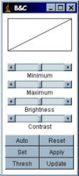

To improve the visualisation of the image, the displayed brightness and contrast can be adjusted with “Image/Adjust/Brightness-Contrast” (hotkey: Shift+C).

The “Auto” applies an intelligent contrast stretch to the way in which the image is displayed. The brightness and contrast is adjusted based on an analysis of the image's (or selection’s) histogram. If pressed repeatedly, it allows a progressively increasing percentage of pixels to become saturated.

Reset changes the “maximum” and “minimum” back to 0 and 255 for 8-bit images and back to the maximum and minimum of the image’s histogram for 16-bit images.

If Auto does not produce a desirable result, select a region of the cell plus some background with a region-of-interest (ROI) tool, then hit the “Auto” button again. It will then do a stretch based on the intensities within the ROI.

Pressing the Apply button permanently changes the actual grey values of the image. Don’t press this button during while analysing image intensity!

If you prefer the image to be displayed as “black on white” rather than “white on black”, the image display can be “inverted” by the command “Image/Color Tables/Invert-LUT”. The command “Edit/Invert…” inverts the pixel values not just the way the image is displayed.

4.2 Getting intensity values from single ROI

If the movie has been opened as a stack, the ROI selected can be analysed with the command: “Plugins/Intensity vs Time Plot” (hotkey: “1”). This generates a single column of numbers - one slice intensity per row.

The top 4 rows of the column are details of the ROI. This is useful to ensure the same ROI isn’t analysed twice and allow relocation of any interesting ROIs. The details are comprised of x-coordinate, y-coordinate, width and height of the ROI. If the ROI is a polyline/freehand ROI rather than a square/oval, the details are given as if the ROI was an oval/square. The (oval)ROI can be restored by entering the details prompted by the “Plugins/Restore ROI” command.

The results are displayed in a plot-window with the ROI details in the plot window title. The plot contains the buttons List, Save, Copy. The Copy button copies the data to the clipboard where it can be pasted into a waiting Excel sheet. The settings for the copy button can be found under “Edit/Options/Plot profile options”. Recommended settings are: Do not save x-values (prevents slice number data being pasted into Excel) and Autoclose (prevents you having to close analysed plot each time.

4.3 Dynamic intensity vs Time analysis

The plugin “Plugins/Stacks – T-functions/Intensity v Time Monitor (this is the Dynamic ZProfile from Kevin (Gali) Baler (gliblr at yahoo.com) and Wayne Rasband simply renamed) ” will update the plot window each time the ROI selection is moved. This may help locate initiation sites of calcium signals for example.

 4.4 Getting intensity values from multiple ROIs

Multiple ROIs can be analysed at once using Bob Dougherty’s “Multi Measure” plugin. There is a native “ROI manager” function which does a similar job except the results generated are not sorted in to columns. Check Bob’s website for updates: http://www.optinav.com/ImageJplugins/list.htm

The Multi Measure plugin that comes with the installation is v3.2.

1. Open t-series.Remove background (See Background correction)

2. It’s worthwhile generating a reference stack to add the ROIs to. Use the “Image/Stacks/Z-project” function (hotkey: Shift+Z)§. Select the “Average” option.

3. Rename this image “Ref expt name” or something memorable.

4. Open “ROI Manager” plugin (“Analyze>Tools>Roi Manager ”
or toolbar icon ).

5. Select ROIs and "Add" to ROI manager (hotkey: t). Clicking "Show All" helps avoid analysing the same cell twice.

6. Once finished selecting ROIs to be analysed in the reference image, you can draw them to the reference image by clicking the "More>>" button and selecting Draw. Save the reference image to the experiment’s data folder and then select the stack to be analysed by clicking on it.

7. Click "More>>" button in the ROI manager and select “Multi” button to measure all the ROIs. Click “Yes” on “Process stack?” dialog. This will put values from each slice in to a single row (multiple columns per slice). Clicking on "Measure" will put all values from all slices and each ROI in a  single column.

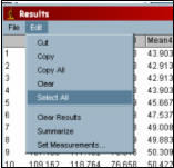
8. Go to “Results” window. Select menu item “Edit/Select All…”. Then “Edit/Copy All”.

9. Go to Excel and paste data. With large data sets this can take some time so check you’re pasting new data in and not the last dataset copied from Multi Measure.

10. To copy ROI co-ordinates in to the Excel spreadsheet, ensure there is an empty row above the intensity data. Got to Multi Measure dialog and click “Copy list” button.

14. Go to Excel, select the empty cell above the first data column and then paste the ROI co-ordinates.

The ROIs can be stored and re-opened later using the Multi Measure dialog button “Save”. Save them in the experimental data folder. The ROIs can be opened later either individually (Multi Measure dialog button “Open”) or all at once (Multi Measure dialog button “Open All”) which opens all the ROIs in a folder.

Oval and rectangular ROIs can also be restored individually from x, y, l, h values using “Plugins/ROI/SpecifyROI…” (hotkey: Shift + G).

4.5. Ratio Analysis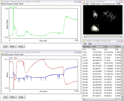

Analysis of dual-channel ratio images requires careful background subtraction prior to analysis. See section 7.5 Background correction. The "Plugins/Stacks - T-functions/Ratio_Profiler" plugin will perform ratiometric analysis of a single ROI on a dual-channel interleaved stack, i.e. the odd-slices are channel 1 images, the even slices channel 2. Perkin Elmer Ultraview and Leica SP dual channel experiments can be directly imported as an interleaved stack using the menu command "File/Import/Image Sequence". If your two channels are opened as separate stacks, e.g. Zeiss, the two channels can be interleaved with the menu command "Plugins/Stacks - Shuffling/Stack Interleaver".

The plugin will generate a green-plot of the ratio values (Ch1÷Ch2 by default; Ch2÷Ch1 if the plugin is run with the Alt-key down); a second plot of the intensities of the individual channels (Ch1 and Ch2); and a results table.

The first row of the results table is the x, y, width and height of the ROI.

From the second row downward, the first column is the time or slice number; the second column the Ch1 mean intensity, Ch2 mean intensity and the ratio value. If the stack has its frame interval calibrated, the "Time" value will be in seconds otherwise it is "Slices". The frame interval can be set for the stack via the menu command "Image/Properties" dialog.

This table can be copied to the clipboard for pasting to another program by using the "Edit/Copy All" menu command.

 

4.5.1 Ratio Analysis Using ROI manager

1. BG subtract the image.

2. Open ROI manager (Analyze/Tools/ROI manager...) and click the "Show All" button.

3. Select the cells to be analysed and add to the ROI manager ("Add" button or keyboard 't' key).

4. Run the plugin "Plugins/Stacks - T-functions/Ratio ROI Manager".

The results window contains the mean  of ch1 and ch2 and their ratio. Each row is a timepoint (slice). The first row contains the ROI details.

To generate a reference image:

1. flatten the stack (Image/Stacks/Zproject" "Projection type: Maximimum"),

2. Adjust the brightness and contrast if required.

3. Ensure the new image is selected and click the "More button" in the ROI manager then select "Label".

 

 

4.6 Obtaining timestamp data

4.6.1 Zeiss LSM

Once imported via the Zeiss LSM panel, the timestamp data can be extracted with the panel’s ‘Apply t-stamp’ button. This will then ask you if you want the timestamp to be added to the image, or displayed in a text file for saving/pasting to excel etc.

4.6.2 Noran

In most instances the x-axis data, i.e. time of each frame, can be calculated from acquisition rates and frame number (e.g. frame 301 acquired with the acquisition rate set to 1 frame per 0.5 seconds was acquired at 25 minutes). However, the acquisition rate is non-linear, in the above experiment frame 301 was actually acquired at 25 minutes 12 seconds. Each frame has stored with it a “timestamp”, the precise time (in nanoseconds!) that it was acquired. This information can be extracted from an opened movie.

The movie must be opened as a stack and the timestamps can be extracted with the command: “Import/Noran timestamp (msec)”  while the Noran Movie is open and selected. The timestamp data appears in the “Results” window. To copy data, click with the right mouse button on the windows, select “Select All”, then right-click again and select Copy. The timestamp data (accompanied by the movie filename) can then be pasted into Excel.

The Noran SGI plugins are not bundled with the ImageJ package. To receive them, please contact tonyc@uhnresearch.ca or their author, Greg Joss <gjoss@bio.mq.edu.au>, Dept of Biology, Macquarie University, Sydney, Australia.

4.6.3 Biorad

This can be accessed via the menu command “Image/Show Info…”. Scroll down and it should give the time at which each slice was acquired. This can be selected, copied in to Excel and the time number obtained by searching and replacing (Excel menu command “Edit/Replace”) the text, leaving only the time data. The “elapsed” time can then be calculated by subtracting row 1 from all subsequent rows.

4.7 Pseudo-linescan

“Linescanning” is a mode of acquisition common to many confocal microscopes where a single pixel wide line is acquired over a period of time instead of the norma1 2-D, x-y image. Usually this allows faster acquisition. The single pixel wide images over the time course are stacked from left to right to generate a 2-D image (i,e, x-t).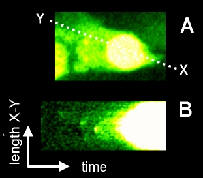

A “pseudo-linescan” is the generation of a linescan-type x-t plot from a 3-D (x, y, t) timecourse and can be useful in displaying 3-D data (x, y, t) in 2 dimensions.

A line of interest must be drawn followed by the command: “Image/Stacks/Reslice” or keyboard “/”. It will prompt for the line width. Enter the width of line you wish to be averaged. A pseudo-linescan “stack” will be generated, each slice representing the pseudo-linescan of a single-pixel wide line along the line of interest. To average the pseudo-linescan “stack”, select “Image/Stack/Z-Project…” and select the Average command. A polyline can be used although this will only allow a single pixel slice to be made.

This example shows the elementary calcium events preceding a calcium wave. HeLa cell loaded with the calcium-sensitive fluorophore, Fluo-3 and imaged whilst responding to application of histamine. A. Frame taken from time-course at the peak of the calcium-release response. (B) The line of pixels along X-Y was taken and stacked side by side from right-to left to generate a "pseudo-line scan". This allows visualisation of the progression of the wave from its initiation site.