Online Manual for the
"ImageJ for Microscopy" collection

6. Colocalisation analysis
Colocalisation analysis is an subject plagued with errors and contention. The literature is full of different methods for colocalisation analysis which probably reflects the fact that one approach does not necessarily fit all circumstances.
Analysis can be considered qualitative or quantitative. However, opinions differ as to which category the different approaches fall!
Qualitative analysis can be thought of as "highlighting overlapping pixels". Although this is often given as a number ("percentage overlap") suggesting quantification, the qualitative aspect arises when the user has to define what is considered "overlapping". The two channels have a threshold set and any areas where they overlap is considered "colocalised". Qualitative analysis has the benefit of being readily understood with little expert knowledge but suffers from the intrinsic user bias of "setting the threshold". There are algorithms available which will automate the thresholding without user intervention but these rely on analysis of the image's histogram which is subject to user intervention during acquisition.
Quantitative analysis removes user bias by analysing all the pixels based on of their intensity (it must be noted that some authors consider this a draw back rather than an advantage due to the intrinsic uncertainty of pixel intensity; see Lachmanovich et al. (2003) J. Microscopy, 212, 122-131). There are a number of coefficients detailed in the literature which can be calculated using ImageJ; each coefficient has it's strengths and weaknesses and should be thoroughly researched before being used. It is this requirement for the coefficient to be fully understood which is a disadvantage when trying to convey information to research peers who are experts in biology, and not necessarily mathematics.
One key issue that can confound colocalisation analysis is bleed through. Colocalisation typically involves determining how much the green and red colours overlap. Therefore it is essential that the green emitting dye does not contribute to the red signal (typically, red dyes do not emit green fluorescence but this needs to be experimentally verified). One possible way to avoid bleed-through is to acquire the red and green images sequentially, rather than simultaneously (as with normal dual channel confocal imaging) and the use of narrow band emission filters. Single and unlabelled controls must be used to assess bleed-through.
6.0 Intensity Correlation Analysis
This plugin generates Mander’s coefficients (see below) as well as performing
Intensity Correlation Analysis as described by Li et al. To fully
understand this analysis you should read:
Li, Qi, Lau, Anthony, Morris, Terence J., Guo, Lin, Fordyce, Christopher B., and
Stanley, Elise F. (2004). A Syntaxin 1, G{alpha}o, and N-Type Calcium Channel
Complex at a Presynaptic Nerve Terminal: Analysis by Quantitative
Immunocolocalization. Journal of Neuroscience 24, 4070-4081.
It is bundled with MBF ImageJ and can be downloaded alone
here.
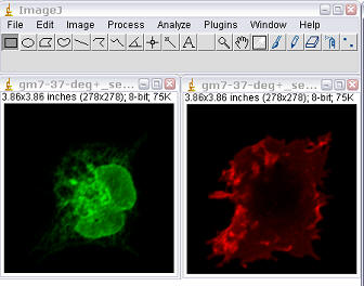
1. Open your two images (File/Open).
2. You must background subtract
each stack:
2a. Select a BG ROI.
2b. Run Plugins/ROI/BG subtract from ROI.
2c. Set threshold if required.
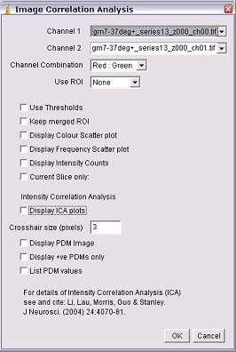
3. Run the ICA plugin (Plugins/Colocalization Analysis/Image Correlation Analysis)
Channel Combination
Select the combination of channel colour, e.g. a TRITC vs FITC analysis would be Red:Green; a FITC vs DAPI would be Green: Blue. This determines the colouring given to the ICA plots and the merged image.
Use ROI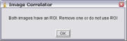
Choose a ROI to analyse from the drop down box. Choose either ‘none’ to anlyse the whole image or “Channel 1:’ to analyse the pixels in both channels within the ROI selected in channel 1.
Use Thresholds
If this is
selected, pixels below the image’s threshold will not be included in the
analysis. For instructions on how to set the threshold, see:
http://rsb.info.nih.gov/ij/docs/menus/image.html#adjust and
http://www.uhnresearch.ca/facilities/MBF/imagej/particle_analysis.htm#threshold
Keep merged ROI
Returns a merged image of the analysed ROI (or full image). The merged colours are determined by the “Channel combination” selected.
DisplaColour Scatter plot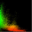
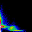
This generates a scatter-plot of red intensities vs green intensities. The colour of the scatter plot pixel represents the actual colour in the image. This does not tell you the frequency of the pixel, but is easier to relate to the original image.
Display Frequency Scatter plot
 The pixels in this scatter-plot
pseudocoloured so that their colour represents the frequency of the red-green
pixel combination in the original image (hot colours representing high values by
convention). This sort of plot contains the most information, but can be a
little difficult to relate it back to the original image.
The pixels in this scatter-plot
pseudocoloured so that their colour represents the frequency of the red-green
pixel combination in the original image (hot colours representing high values by
convention). This sort of plot contains the most information, but can be a
little difficult to relate it back to the original image.
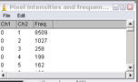 Display intensity counts
This generates a text window with the red intensities, green intensities and frequency of the intensity pairs. This can be exported to a spreadsheet program for further analysis.
Current Slice Only
Select this if you do not wish to analyse the whole stack. Only the current slice in the Channel 1 stack (and the corresponding slice in the green channel) will be analysed.
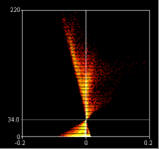
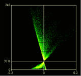
Display ICA plots
When checked this option draws two plots, one for the red channel one for the green. The axes on the plots are the PDM values on the x-axis and the red or green intensity on the y-axis.
The PDM value is the Product of the Differences
from the Mean, i.e. for each pixel:
PDM = (red intensity- mean red
intensity)×(green intensity – mean green intensity)[1]
Crosshair size (pixels)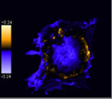
The points of the ICA plots are plotted as cross-hairs. You can select the size of the crosshair here.
Display PDM image
This option generates a new image where each pixel is equal to the PDM value at that location. The Image is pseudocoloured and a PDM scale bar is inserted.
For clarity, pixels that are below average in both channels are excluded.
 Display +ves only
This option will generate a 2 slice stack. The first images pixels are the positive PDM values resulting from both pixels above the mean (i.e. red intensity-mean red intensity and green intensity-mean green intensity are both positive). The second slice are pixels that have pixel values in each channel which are both below the mean (i.e. red intensity-mean red intensity and green intensity-mean green intensity are both negative).
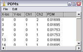
List PDM values
This generates a list of PDM values that can be exported to spreadsheet programs for further analysis.
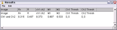
Results Window
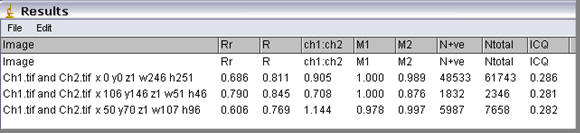
If the Results window is closed or does not contain ICA data then the plugin will enter a “Header” row then the data row. The second time the plugin is run only the data row is entered. The column information is detailed below.
Image
The name of the images and the ROI that has been analysed is entered in the Image column. If no ROI was selected of the “Use ROI” option unchecked then the ROI describes the image dimensions.
Rr
This is the Pearson’s correlation coefficient. Zero-zero pixels are not included in this calculation.
This is a popular method of quantifying correlation in many fields of research from psychology to economics. In many forms of correlation analysis the values for Pearson’s will range from 1 to -1. A value of 1 represents perfect correlation; -1 represents perfect exclusion and zero represents random localisation. However, this is not the case for images. While perfect correlation gives a value of 1, perfect exclusion does not give a value of -1. Low (close to zero) and negative values for Pearson’s correlation coefficient for fluorescent images can be difficult to interpret. However, a value close to 1 does indicate reliable colocalisation.
R
This is Mander’s Overlap coefficient. This is easier than the Pearson’s coefficient to comprehend. It ranges between 1 and zero with 1 being high-colocalisation, zero being low. However, the number of objects in both channel of the image has to be more or less equal.
Ch1:Ch2
This value represents the red: green pixel ratio. The Overlap coefficient (R) is strongly influenced by the ratio of red to green pixels and should only be used if you have roughly equal numbers of red and green pixels (i.e. Nred ÷ Ngreen pixels ~1).
M1 and M2
These split coefficients are Mander’s Colocalization coefficients for channel 1 (M1) and channel 2 (M2).
These split-coefficients avoid issues relating to absolute intensities of the signal, since they are normalised against total pixel intensity. We also get information as to how well each channel overlaps the other. There are cases where red may overlap significantly with green, but most of the may not overlap with the red.
If the assumption is made that greyscale number equates to dye molecules (this is not necessarily correct) then these coefficients represent the percentage of red dye molecules that share their location with a green dye molecule.
These coefficients are very sensitive to poor background correction and do not take in to account the intensity of the second channel, other than it is non-zero. For example, a bright red pixel colocalising with a faint green pixel is considered equivalent to a bright red pixel colocalising with a bright green pixel. Intuitively, a red-green pixel-pair of similar intensities should be considered “more colocalised” than a pixel pair of widely differing intensities.
N+ve
This represents the number of pixel pairs that have a positive PDM value.
Ntotal
This is the number of pixels pairs in the images that where at least one of the pixel pairs is above zero..
ICQ
This is the Intensity Correlation Quotient. If the intensities in two images vary in synchrony (i.e. they are dependent), they will vary around their respective mean image intensities together. So, if a pixel’s intensity is below average in the red channel (i.e. Ri-Rmean< 0); it will be below average in the green channel (i.e. Gi-Gmean<0). Similarly, if a pixel is above average in one channel it will be above average in the other. Therefore, in an image where the intensities vary together, the product of the differences from the mean (PDM), will be positive. The converse is true. If the pixel intensities vary asynchronously, i.e. the channels are segregated so that when a red pixel is above average, the corresponding green pixel is below average; then most of the PDMs will be negative.
The ICQ is based on the non-parametric sign-test analysis of the PDM values and is equal to the ratio of the number of positive PDM values to the total number of pixel values. The ICQ values are distributed between -0.5 and +0.5 by subtracting 0.5 from this ratio.
Random staining: ICQ~0; Segregated staining: 0> ICQ³ -0.5; Dependent staining: 0<ICQ£+0.5
[1] PDM is equal to the value (A-a)*(B-b) as described in Li et al. 2004.
6.1 Manders' Coefficients
6.1.1 “Manders' Coefficient" (formerly Image Correlator plus ” and “Red-Green Correlator” plugins)
This plugin generates
various colocalisation coefficients for two 8 or 16-bit images or stacks.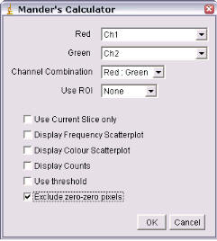
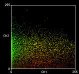
The plugins generate a scatter plots plus correlation coefficients. In each scatter plot, the first (channel 1) image component is represented along the x-axis, the second image (channel 2) along the y-axis. The intensity of a given pixel in the first image is used as the x-coordinate of the scatter-plot point and the intensity of the corresponding pixel in the second image as the y-coordinate.
The intensities of each pixel in the “Correlation Plot” image represent the frequency of pixels that display those particular red/green values. Since most of you image will probably be background, the highest frequency of pixels will have low intensities so the brightest pixels in the scatter plot are in the bottom left hand corner – i.e. x~ zero, y ~ zero. The intensities in the “Red-Green correlation plot” image represent the actual colour of the pixels in the image.
Mito-DsRed; ER-EGFP
|
Pearson's correlation (R)=0.34 Overlap coefficient (R)=0.40 Nred ÷ Ngreen pixels=0.66 Colocalisation coefficient for red (Mred)=0.96 Colocalisation coefficient for green (Mgreen)=0.49 |
|
|
|
|


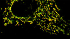
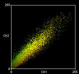
TMRE (red) plus Mito-pericam (Green)
|
Pearson's correlation Rr=0.93 Overlap coefficient R=0.94 Nred ÷ Ngreen pixels=0.93 Colocalisation coefficient (red) Mred=0.99 Colocalisation coefficient (green) Mgreen=0.98 |
|
|
|
|

Both plugins generate various colocalisation coefficients: Pearson’s (Rr), Overlap (R) and Colocalisation (M1, M2) See Manders, E.E.M., Verbeek, F.J. & Aten, J.A. ‘Measurement of co-localisation of objects in dual-colour confocal images’, (1993) J. Microscopy, 169, 375-382. See tutorial sheet ‘Colocalisation’ for details. The threshold is also reported (0,0 means no threshold was used).
6.2 Colocalisation Test
When a coefficient is calculated for two images, it is often unclear quite what this means, in particular for intermediate values. This raises the following question: how does this value compare with what would be expected by chance alone?
There are several approaches that can be used to compare an observed coefficient with the coefficients of randomly generated images. Van Steensel (3) adopted an approach where the observed colocalisation between channel 1 and channel 2 was compared to colocalisation between channel 1 and a number of channel 2 images that had been translated (i.e. displaced by a number of pixels) in increments along the image’s X-axis. Fay et al (4) extended this approach by translating channel 2 in 5-pixel increments along the X- and Y-axis (i.e., –10, –5, 0, 5, and 10) and ± 1 slices in the Z-axis. This results in 74 randomisations (plus one original channel 2). The observed correlation was compared to these 74 and considered significant if it was greater than 95% of them.
Costes et al. (5) subsequently adopted a different approach, based on “scrambling” channel 2. The original channel 1 image was compared to 200 “scrambled” channel 2 images; the observed correlations between channel 1 and channel 2 were considered significant if they were greater than 95% of the correlations between channel 1 and scrambled channel 2s.
Costes’ scrambled images were generated by randomly rearranging blocks of the channel-2 image. The size of these blocks was chosen to equal the point spread function (PSF) of the image.
An approximation of Costes’ approach is used by Bitplane’s Imaris and also the Colocalisation Test plugin. For Imaris, a white noise image is smoothed with a Gaussian filter the width of the image’s PSF. The Colocalisation Test plugin generates a randomized image by taking random pixels from the channel-2 image; it then smoothes the image with a Gaussian filter, which is again the width of the image’s PSF.
The Colocalisation Test plugin calculates Pearson’s correlation coefficient for the two selected channels (Robs) and compares this to Pearson’s coefficients for channel 1 against a number of randomized channel-2 images (Rrand).
Using the Plugin
ROI or Mask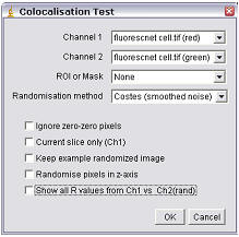
Select the ROI you wish to analyze. You can choose “None,” “ROI in channel 1,” or “ROI in channel 2.” If an ROI is selected, but one is not present, then no ROI will be used. Alternatively, an image can be selected as a mask. Only pixels in channel 1 and channel 2 that correspond to a non-zero value in the mask will be included in the calculations.
Randomization Method
The options here are either “Fay (translation)” or “Costes (smoothed noise)” or “van Steensel (x-translation)”. If “Costes” is selected, a second dialog will open after the first is “okayed”; this allows the user to define the PSF width and whether pixels are randomized in the Z-axis also.
Ignore zero-zero pixels
If this is checked, then pixels with a value of zero in both channels will be ignored as background. Checking this option generates values that more closely resemble those generated by Imaris (with no mask).
Current Slice only (Ch1)
If you choose two stacks, but wish only to analyze the current slice, selecting this option will compare the current slice of channel 1 with its corresponding slice in channel 2.
Keep example randomized image
Select this if you wish to keep a single example of a randomized image (or a stack if it a stack analysis).
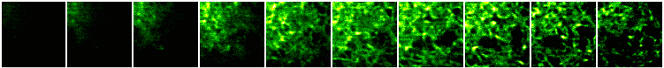
|
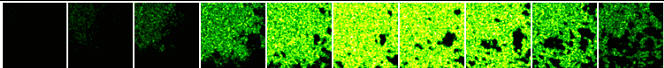
Montage of z-slices from a raw channel 2 image (ER-GFP expressing HeLa cell) |
|
|
|
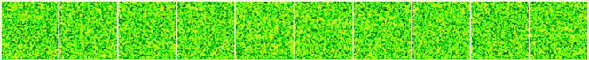
Montage of z-slices from an example randomized image that has been randomized in x, y AND z. |
|
|
|
Montage of z-slices from an example randomized image that has been randomized in x, y only. |
|
|
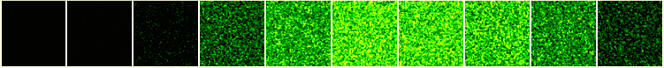
|
Montage of z-slices from an example randomized image that has been randomized in x, y only and with ch2 selected as a mask. |
|
|
Randomising in the z-axis generates data that is more consistent with that of Imaris. For example: ER-Mito.tif (red) and ER-Mito.tif (green)
|
Randomisation of Ch2 |
R(obs) |
R(rand) mean±sd |
%(Ro>Rr) |
Iterations |
Randomisation |
PSF width |
|
Costes X, Y,Z |
0.357 |
0.002±0.003 |
100% |
10 |
Costes X, Y, Z |
0.514 µm |
|
Costes X, Y |
0.357 |
0.477±0.001 |
0% |
10 |
Costes X, Y |
0.514 µm |
|
Imaris |
0.357 |
|
1.00 |
|
|
0.514 µm |
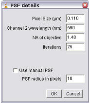 PSF
details
PSF
details
If you have opted for Coste’s method of randomization, a second dialog will appear.
Randomize pixels in z-axis
For a single slice image this option does nothing. For stacks randomized with Costes’ approach this option will activate randomization in z as well as in x and y. When this is unchecked, random pixels are taken from a channel 2 slice and put in the same slice in the randomized channel 2 images. If this option is checked, the minimum and maximum pixel intensities in the stack are calculated, and random values in this range are added to each slice.
Pixel Size (µm)
Enter the pixel size here. If the image is properly calibrated then the dialog pulls the correct value from the image.
Channel wavelength (nm)
Enter the central emission wavelength of channel 2. This is typically an approximation; for traditional “red-dyes” this will be about 590 nm.
NA of objective
Enter the numerical aperture of the objective used to acquire the image
Iterations
Enter the number of randomizations you wish to perform. The higher this number is the more accurate the data, but it will also take longer to calculate. This is an especially important factor to consider in stack analysis.
Manual PSF
The above information (pixel size, wavelength, NA) is used to calculate the appropriate size for the Gaussian filter. You can override this, or if you do not know the appropriate settings then check the “Use Manual PSF” option and enter the PSF radius in pixels. Note: entering a value too small may result in positive colocalisation where there is none. See Costes’ supplemental material
Results
Data generated with the following options: No ROI; Costes Randomization; Randomized in X and Y only.
|
Filename |
Robs |
Imaris R |
Rrand (mean±sd) |
Robs>Rrand |
Imaris P |
Iterations |
Randomization |
PSF width |
|
BBB_rgb |
0.002 |
0.002 |
0.002±0.004 |
54% |
0.602 |
10 |
Costes |
0.505 µm (5 pix.) |
|
Biofilm.lsm |
0.801 |
0.801 |
0.001±0.001 |
100% |
1.00 |
10 |
Costes |
0.544 µm (3 pix.) |
|
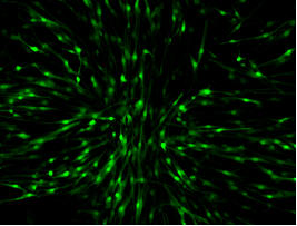
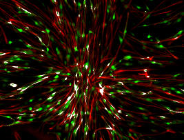
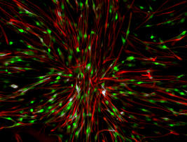
fluorescent cells |
0.363 |
0.363 |
-0.001±0.002 |
100% |
1.00 |
10 |
Costes |
0.884 µm (1 pix.) |
|
Nestin_GFP.tif |
0.256 |
0.256 |
-0.000±0.000 |
100% |
1.00 |
10 |
Costes |
0.884 µm (1 pix.) |
|
Syntaxin RGB |
0.617 |
0.617 |
0.005±0.014 |
100% |
1.00 |
10 |
Costes |
0.505 µm (5 pix.) |
|
ERMito stack |
0.398 |
0.398 |
0.464±0.001 |
0% |
1.00 |
10 |
Costes |
0.505 µm (5 pix.) |
|
ERMito ZProjection |
0.048 |
0.048 |
0.012±0.020 |
100% |
1.00 |
10 |
Costes |
0.505 µm (5 pix.) |
Robs = Pearson's
coefficient for ch1 v ch2;
Rrand = Pearson's coefficient for ch1 vs randomised ch2;
6.3 Colocalisation Threshold
Background
This performs analysis based on the approach of Costes et al ). Implementations of this approach can also be found in Bitplane’s Imaris and NIH’s MIPAV software.
The function of this approach is to determine automatically a threshold for each channel. Pixels below this threshold are ignored for the purposes of the colocalisation quantification.
The threshold is determined in two stages. First, an orthogonal regression is performed on the image’s scatterplot. Then, a threshold is stepped down along this regressed line. Pixels below this threshold are included in the calculation of Pearson’s coefficient. When Pearson’s coefficient equals zero, the threshold for subsequent calculations has been found.
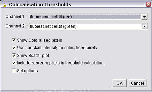
Using the Plugin
Show Colocalised Pixels
 This
results in the generation of a new greyscale image including only the
colocalised pixels (i.e., in which both channel 1 and channel 2 are above their
respective thresholds).
This
results in the generation of a new greyscale image including only the
colocalised pixels (i.e., in which both channel 1 and channel 2 are above their
respective thresholds).
Use constant intensity for colocalised pixels
This option allows the image of colocalised pixels to be white; otherwise the pixel intensity will equal √(Ch1×Ch2).
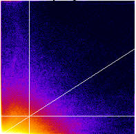
Show Scatterplot
This will generate a scatterplot (channel 1 along the x-axis; channel 2 along the y-axis) with both the linear regression line as well as the thresholds marked.
Include zero-zero pixels in threshold calculation
This option allows inclusion/exclusion of zero-zero pixels in the calculation of the thresholds. Including the zero-zero pixels results in calculated thresholds similar to Imaris; excluding them generates thresholds similar to those determined by MIPAV.
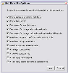
Set Options
When clicked, this option activates the Results Options dialog (see below), and allows you to choose results are reported. By default, all results are reported. (The plugin should remember your preferences.) Other options can be easily added; contact Tony Collins for help with this.
|
Channel 1 |
Channel 2 |
|
Colocalisation Image:
Constant Intensity |
Colocalisation Image:
Variable Intensity |
|
Scatter plot generated |
|

Results Options
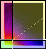 The
scatterplot generated can be thought of as consisting of four quadrants (shown
in the scatter plot diagram as red, green, blue, and yellow).
The
scatterplot generated can be thought of as consisting of four quadrants (shown
in the scatter plot diagram as red, green, blue, and yellow).
Red quadrant = (Ch2>Ch2 threshold)&(Ch1<Ch1 threshold) = Ch2 above; Ch1 below;
Green quadrant = (Ch2<Ch2 threshold)&(Ch1<Ch1 threshold) = Ch1 below; Ch2 below;
Blue quadrant = (Ch2<Ch2 threshold)&(Ch1>Ch1 threshold) = Ch1 above; Ch2 below;
Yellow quadrant = (Ch2>Ch2 threshold)&(Ch1>Ch1 threshold) = Ch1 above; Ch2 above;
Show Linear Regression Solution – m; b
Returns the result of the orthogonal regression: Ch2 = (Ch1*m) + b.
Show thresholds – Ch1 thresh; Ch2 thresh
Returns each threshold. Pixels below this threshold have a Pearson’s correlation coefficient of ~ zero. (Red + Green + Blue areas in Scatterplot 1).
Pearson’s for Whole image – Rtotal
 Returns
Pearson’s correlation coefficient for all the non zero-zero pixels in the image
(ignores regression options).
Returns
Pearson’s correlation coefficient for all the non zero-zero pixels in the image
(ignores regression options).
Pearson’s for image above thresholds – Rcoloc
Returns Pearson’s correlation coefficient for pixels where both Ch1 and Ch2 are above their respective threshold (yellow area in Scatterplot 1).
Pearson’s for image below thresholds – Ch1 thresh; Ch2 thresh
Returns Pearson’s correlation coefficient for pixels where either Ch1 or Ch2 are below their respective threshold (i.e., the Red + Green + Blue areas in Scatterplot 1). This indicates how well a threshold has been set. This value should be close to zero.
Mander’s Original coefficient – M1; M2
This generates a value for each channel. These are the colocalisation coefficients as described originally by Manders et al These coefficients do not set a threshold other than “greater than zero.”
Mander’s using thresholds – tM1; tM2
This generates a value for each channel. This is a modification of Mander’s original formula, except the thresholds that have been calculated are used.
Number of colocalised voxels – Ncoloc
This is the number of voxels which have both channel1 and channel 2 intensities above threshold (i.e., the number of pixels in the yellow area of the scatterplot).
%Image volume colocalised – %Volume
This is the percentage of voxels which have both channel 1 and channel 2 intensities above threshold, expressed as a percentage of the total number of pixels in the image (including zero-zero pixels); in other words, the number of pixels in the scatterplot’s yellow area ÷ total number of pixels in the scatter plot (the Red + Green + Blue + Yellow areas).
%Voxels Colocalised – %Ch1 Vol; %Ch2 Vol
This generates a value for each channel. This is the number of voxels for each channel which have both channel 1 and channel 2 intensities above threshold, expressed as a percentage of the total number of voxels for each channel above their respective thresholds; in other words, for channel 1 (along the x-axis), this equals the (the number of pixels in the Yellow area) ÷ (the number of pixels in the Blue + Yellow areas). For channel 2 this is calculated as follows: (the number of pixels in the Yellow area) ÷ (the number of pixels in the Red + Yellow areas).
%Intensity Colocalised – %Ch1 Int; %Ch2 Int
This generates a value for each channel. For channel 1, this value is equal to the sum of the pixel intensities, with intensities above both channel 1 and channel 2 thresholds expressed as a percentage of the sum of all channel 1 intensities; in other words, it is calculated as follows: (the sum of channel 1 pixel intensities in the Yellow area) ÷ (the sum of channel 1 pixels intensities in the Red + Green + Blue + Yellow areas).
%Intensities above threshold colocalised – %Ch1 Int > thresh; %Ch2 Int > thresh
This generates a value for each channel. For channel 1, this value is equal to the sum of the pixel intensities with intensities above both channel 1 and channel 2 thresholds expressed as a percentage of the sum of all channel 1 intensities above the threshold for channel 1. In other words, it is calculated as follows: (the sum of channel 1 pixel intensities in the Yellow area) ÷ (sum of channel 1 pixels intensities in the Blue + Yellow area)
Sample Results
|
Image |
Software |
%Vol |
%Ch1 |
%Ch2 |
ThreshCh1 |
ThreshCh2 |
|
BBB_rgb |
MIPAV |
No threshold determined |
||||
|
Imaris |
0.0 |
2.4 |
0.4 |
252 |
7 |
|
|
ImageJ (excl. 00*) |
0.0 |
0 |
0 |
255 |
7 |
|
|
ImageJ (incl. 00) |
0.0 |
0 |
0 |
255 |
7 |
|
|
Biofilm |
MIPAV |
41.6 |
99.7 |
81.5 |
2 |
26 |
|
Imaris |
45.0 |
99.8 |
84.4 |
1 |
21 |
|
|
ImageJ (excl. 00) |
40.2 |
99.4 |
75.3 |
3 |
26 |
|
|
ImageJ (incl. 00) |
40.2 |
99.4 |
75.3 |
3 |
26 |
|
|
Fluorescent cells** |
MIPAV |
7.9 |
33.2 |
36.1 |
74 |
51 |
|
Imaris |
56.1 |
83.9 |
98.3 |
11 |
5 |
|
|
ImageJ (excl. 00) |
6.8 |
16.2 |
22.5 |
77 |
51 |
|
|
ImageJ (incl. 00) |
53.3 |
79.7 |
96.7 |
13 |
6 |
|
|
Nestin_GFP |
MIPAV |
5.2 |
32.4 |
30.3 |
63 |
39 |
|
Imaris |
14.9 |
47.3 |
53.9 |
36 |
23 |
|
|
ImageJ (excl. 00) |
5.5 |
18.6 |
21.0 |
61 |
38 |
|
|
ImageJ (incl. 00) |
13.0 |
34.4 |
40.5 |
38 |
24 |
|
|
ER-Mito Z-series |
MIPAV |
8.8 |
44.3 |
39.4 |
15.3 |
20 |
|
Imaris |
22.8 |
66.1 |
59.6 |
8 |
10 |
|
|
ImageJ (excl. 00) |
8.2 |
39.5 |
37.6 |
15 |
20 |
|
|
ImageJ (incl. 00) |
18.1 |
62.1 |
53.8 |
9 |
12 |
|
|
Syntaxin RGB |
MIPAV |
51.4 |
91.9 |
92.7 |
11 |
8 |
|
Imaris |
60.0 |
92.8 |
95.1 |
9 |
6 |
|
|
ImageJ (excl. 00) |
50.7 |
84.3 |
90.1 |
11 |
8 |
|
|
ImageJ (incl. 00) |
53.3 |
86.1 |
91.4 |
10 |
6 |
|
* Including (incl. 00) or excluding (excl. 00) zero-zero pixel pairs for calculation of the thresholds.
** There is considerable background in this image. See ImageJ sample “File/Open Samples/Fluorescent Cells”.
Users of Imaris are encouraged to use a third channel mask in their analysis: this would, in effect, exclude zero-zero pixels. For the purposes of the comparison above, no mask channel was used with Imaris or ImageJ. Below is a table of results using the mask option of ImageJ and Imaris for the Nestin_GFP example image.
|
File |
Software |
Mask |
Ch1 Threshold |
Ch2 Threshold |
|
Nestin_GFP |
Imaris |
Ch1 |
76 |
46 |
|
ImageJ |
Ch1 |
77 |
47 |
|
|
Imaris |
Ch2 |
60 |
41 |
|
|
ImageJ |
Ch2 |
61 |
42 |
6.4 Highlighting Overlapping pixels
6.2.1
“Colocalization” plugin 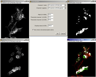
Plugins/Colour functions/Colocalization . This plugin will generate an image of colocalised pixels and also an image of those colocalised pixels superimposed on a RGB-merge of two 8-bit images. This type of colocalisation requires users to decide a “threshold” value which can introduce bias.
This plugin highlights the colocalised points of two 8-bits images (or stacks). The colocalised points will appear white by default (Display value = 255). The plugin merges the red and green 8-bit channels to an RGB image and highlights the colocalised pixels in white. Pixels are considered colocalised if their intensities are higher than the threshold of their channels (set at 50 by default): and if the ratio of their intensity is higher than the ratio setting value (set at 50% by default). A second image of just the white colocalised pixels is generated if the “Also show colocalised pixels alone” option is checked
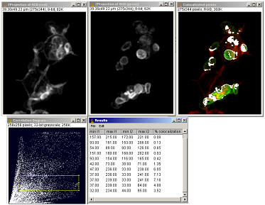
6.2.2 “Colocalization finder” plugin
 Menu command “Plugins/Stacks – RGB
functions/Colocalization finder
”
Menu command “Plugins/Stacks – RGB
functions/Colocalization finder
”
This plugin will prompt you for two grey-scale images and creates a scatter plot and a red-green merged image. The pixels represented by the scatter plot point can be highlighted by selecting the points with the rectangular selection tool only. The 32-bit scatter plot is best visualised after having had its contrast stretched (“Image/Adjust/Brightness&Contrast…”)