Online Manual for the
MBF-ImageJ collection

7 Image intensity Processing
7.1 Brightness and Contrast
|
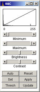
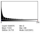
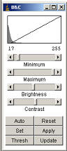
The Brightness and Contrast window (Hotkey: Shift+C; menu command “Image/Adjust/Brightness and Contrast…”) will allow you to change the way the image is displayed. The x-axis of the plot represents the pixel intensities in the image; the y-axis represents the intensity that they are displayed (bottom of y-axis is display black; top is display white). Initially, there is a linear relationship between the image intensity and the display intensity. Increase the minimum value to display your image background as black (i.e.) zero and decrease the maximum value to display the brightest objects in your image as white. This is best achieved in a greyscale image by loading the “HiLo LUT” (“Plugins/LUT/Hi Lo Indicator…”; hotkey: F1). The Auto button applies a linear histogram stretch (a.k.a. Normalisation), i.e. it sets the displayed value to match the maximum and minimum intensity in the image. Clicking the Auto button again will allow increasing amounts of saturation. By clicking the Apply button the values in the image are changed to match their displayed value. Do not do this prior to quantifying intensity values! If you are processing a stack, you will be given the option to apply this adjustment to the entire stack. If Auto does not produce a desirable result, select a region of the cell plus some background with an ROI tool, then hit the Auto button again. It will then do a stretch based on the intensities within the ROI. If you prefer the movie to be displayed as “White and Black” rather than “Black and White”, the image display can be “inverted” by the command “Image/Color Tables/Invert-LUT”. The command “Edit/Invert…” inverts the pixel values not just the way the image is displayed. |
|
7.2 Non-linear contrast stretching
7.2.1 Equalization
|
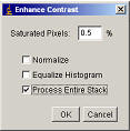
More control of the brightness and contrast adjustment can be achieved with the “Process/Enhance contrast” menu command. Here, when applied to a stack, it applies the adjustment based on each slice’s histogram, not just the one currently displayed as is done with the Brightness and Contrast window. “Equalisation” applies a non-linear stretch of the histogram based on the square root of the intensity (see online guide to image processing: http://www.dai.ed.ac.uk/HIPR2/histeq.htm). The “Normalize” option performs a simple linear stretch on the image in a similar way to the “Auto” option in the Brightness and Contrast window, except that when applied to a stack each slice in stack is adjusted differently based on the slice’s histogram. |
|
7.2.2 Gamma
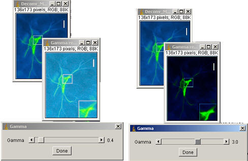
This can be though of as a non-linear histogram adjustment. Faint objects can be made more intense without saturating bright objects (gamma <1). Similarly, medium-intensity objects can be made fainter without dimming the bright objects (gamma > 1). The intensity of each pixel is “raised to the power” of the gamma value and then scaled to 8-bits or the min and max of 16-bit images.
For 8 bit images; New intensity = 255 × [(old intensity÷255) gamma]
Gamma can be adjusted via the “Process/Math/Gamma” command or the “Plugins/Utilities/Gamma Scroll-bar” plugin. The latter will open up a new window copy of your image and you can adjust the gamma with the scroll bar. Click on “Done” when you are finished. This is a bit flaky and doesn’t react well if you change images in mid-adjust! This does not work on stacks. You can use the Scroll-bar to determine the desired gamma value on one slice of your stack, and then apply this gamma value to the stack via the “Process/Math/Gamma” command.
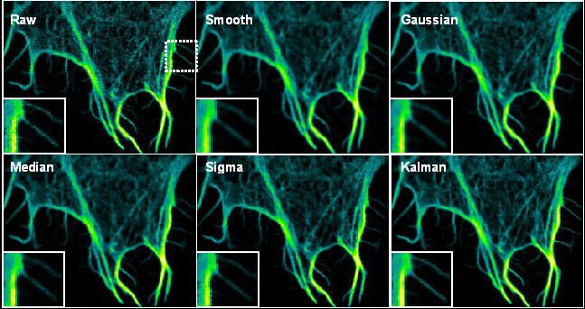
7.4 Filtering
See the online reference: http://www.dai.ed.ac.uk/HIPR2/filtops.htm for a simple explanation of digital filtering.
Filters can be found under the menu item “Process/Filters...”. Typically use a “Radius (pixels)” of 1 which equates to a 3×3 “kernel” – see online reference.
Mean filter: the pixel is replaced with the average of it and its neighbours within the radius. The menu item “Process/Smooth” is a 3×3 mean filter.
Gaussian filter: The is similar to smoothing but replaces the pixel with a pixel of value proportional to a normal distribution of it’s neighbours – not explained well, I know, but you’ve probably skipped the online reference and you need to read that to understand the way the filter works properly.
Median filter: the pixel is replaced with the median of it and its adjacent neighbours. This removes noise and preserves boundaries better than simple mean filtering, but can look odd. (The menu item “Process/Noise/Despeckle” is a 3×3 median filter).
Kalman filter : Sophisticated filtering for time-course experiments – a sort of “weighted running average”. Best used if the sample frequency is higher than the “event” frequency i.e. slowly occurring events. Otherwise you get odd, blurry results. “Process/Filter/Kalman Stack…”.
Sigma filter: A modification on the standard mean filter but preserves edges better – can be though of as a “gentle smooth”. The user specifies the kernel size, the Sigma width and the minimum number of pixels to include. A Sigma value for the kernel is calculated (based on the variance and mean of the intensities) and only pixels within this Sigma range (= Sigma × the user defined Sigma Width scaling factor) are used to calculate the mean. If there are too few pixels (exact number set in the user dialog: Minimum number of pixels) in the kernel that are within the Sigma range then the central pixel which is assumed to be spuriously low or high and the mean of the rest of the kernel is taken. Increasing the Sigma width and the minimum number of pixels results in increased smoothing and loss of edges. This plugin is under development, please send me any feedback. “Process/Filter/Sigma Filter…” J.S. Lee, Digital Image Smoothing and the Sigma Filter, Computer Vision, Graphics, and Image Processing 24, (1983) p. 255-269.
Anisotropic Diffusion. This is an edge preserving smoothing filter.
7.5 Background correction
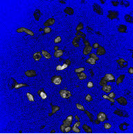
Background correction can be done in several ways and is facilitated if the grey image has the “Plugins/LUT/Hi Lo indicator” (Hotkey: F1) LUT loaded. This displays the zero values blue and the 255 white values red.
If the background is relatively even across the image, it is most simply remove with the Brightness&Contrast command – slowly raise the Minimum value until most of the background is displayed blue. The press the Apply button to change the grey-values and remove the background.
7.5.1 Rolling-Ball background correction
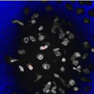
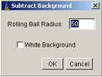
For uneven background the menu command “Process/Subtract background” can be used. This menu command removes uneven background from images using a “rolling ball” algorithm. The radius should be set to at least the size of the largest object that is not part of the background. It can also be used to remove background from gels where the background is white. Running the command several times may produce better results.
|
RAW |
|
“Process/Subtract Background…” |
|
|
|
|
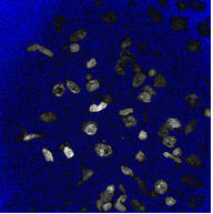
Once the background has been evened, final adjustments can be made with the Brightness&Contrast control.
|
|
|
|
7.5.2 ROI background correction
The rolling-ball algorithm is time consuming. If the background is even across the field of view it is possible to select a background region of interest and subtract the mean value of this area for each slice from each slice. Use the selection tools to select an area of background and run the menu command “Plugins/ROI/BG Subtraction from ROI”. This macro will subtract the mean of the ROI from the image plus an additional value equal to the standard deviation of the ROI multiplied by the scaling factor you enter (3 by default).
i.e. it subtracts [mean + (sd×scalingfactor)]
This macro also works with stacks and so can be used with time-courses with varying background.
|
Before correction |
Background intensity over time |
After “ROI_BG_Correction” |
|
|
|
|
7.1 Flat-field correction
7.1.1 Proper correction
This technique is applied to brightfield images. Uneven illumination, dirt/dust on lenses can result in a poor quality image. This can be corrected by acquiring a “flat-field” reference image with the same intensity illumination as the experiment. The flat field image should, ideally, be a field of view of the coverslip without any cells/debris. This is often not possible with the experimental coverslip, so a fresh coverslip may be used with approximately the same amount of buffer as the experiment. With fixed-specimens try removing the slide completely
|
|
||
|
RAW |
Flat-field |
Processed |
|
|
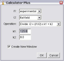
1. Open both experimental image and flat-field image. 2. “Select all” of the flat-field image (hotkey: A) and measure the average intensity (hotkey: M). This value will appear in the results window and represents your k1 value below. 3. Use the “Image Calculator plus” plugin (“Analyse/Tools/Calculator plus” ). 4. i1 = experimental image; i2 = flat-field image; k1 = mean flat-field intensity; k2 = 0. Select the "Divide" operation. This can also be done using the “Process/Image Calculator” function and ensuring the “32-bit Result” option is checked. You will then need to adjust the brightness and contrast and change the image to 8-bit.
|
7.1.2 Pseudo-correction
|
The menu command “Process/Filters/Pseudo-flat field ” automates this process. You are prompted to enter the kernel size for the mean filter; try the default value of 50 first. You can opt to keep the flat field image open to check whether the kernel is large enough. The objects should not be visible in the flat field image. This can also be used with stacks for brightfield time-courses that vary in intensity with time. This is time consuming though. |
|
|
|
The first RAW image (top) pseudo-flat field corrected. Here the pseudo-flat field corrects for the uneven illumination but does not correct the dust specks. Compare this with the result of a proper flat-field correction above. |
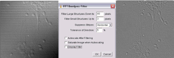
7.1.3 FFT background correction
We sometimes see uneven illumination and also horizontal "scan lines" in transmitted light images acquired with confocal microscopes. This background can be corrected using the native FFT bandpass function (Process/FFT/Bandpass...).
Experiment with the settings to optimise the filtering.
7.2 Masking unwanted regions
7.2.1 Simple masking
Draw around the area you want with one of the ROI tools then use: “Edit/Clear outside”. This will change area outside the selected region to the background value.
7.2.2 Complex masking
A more sophisticated masking can be done by “thresholding” the image and subtracting this new binary image from the original.
1. Duplicate the image (if it’s a stack it’s worthwhile generating a “average projection” of a few frames).
2. Threshold this image using the menu command “Image/Adjust/Threshold” (hotkey Shift+T).
3. Hit the Auto button and then adjust the sliders until cells are all highlighted red.
4. Then click “Apply”. Check the tick box: “black foreground, white background”. You should now have a white and black image with your cells black and background white. If you have white cells and black background, invert the image with “Edit/Invert”.
5. This can be smoothed (“Process/Smooth”) and the black area enlarged slightly with “Process/Binary/Dilate” to give a better mask
6. Using the regular Image calculator “Process/Image calculator” subtract this black and white “mask” image from your original image/stack.