The content of this page has not been vetted since shifting away from MediaWiki. If you’d like to help, check out the how to help guide!
General
With NanoTrackJ it is possible to analyze videos of diffusing particles. It is mainly tested with tracking moving diffraction patterns of diffusing nanoparticles. The plugin estimates the particle size and diffusion coefficient distribution. Therefore, a fundamental relationship between the diffusion coefficient and the hydrodynamic diameter is exploited: The Stokes-Einstein relation.
If you are using NanoTrackJ in a scientific publication, please cite:
Wagner, T., Lipinski, H.-G. & Wiemann, M., 2014. Dark field nanoparticle tracking analysis for size characterization of plasmonic and non-plasmonic particles. Journal of Nanoparticle Research, 16(5), p.2419.
Parameters
Center Estimation: here are three methods available. The blob method requires a binary image. The objects you want to track should be connected foreground pixels. Such connected regions are often called “blobs”. Each blob represents a particle to be tracked. You have to segment your image (e.g. through thresholding) to use this method. The centroid of the blob is used for tracking.
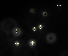
The maxima method utilizes the Process › Find Maxima method of ImageJ. A “Spot Assistant” helps the user to select an appropriate mean filter size and tolerance value.
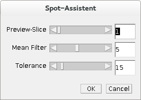
This is the recommended method and it is also usable with RGB image series. The found maxima are used as centroids to track the particles.

The maxima method & gaussian fit also utilizes the Process › Find Maxima method of ImageJ but do an gaussian fit after that to improve the estimation qualtity. Theoretically it achieves sub-pixel accuracy. However, diffraction patterns often suffers from saturation and sometimes they do not even have a gaussian shape so that sub-pixel accuracy is not achievable.
Diffusion-Coefficient-Estimator: Two methods are available: The regression method and the covariance method. The regression method is the most used in literature to estimate the diffusion coefficient. It evaluates the mean squared displacement for different time lags. Then it fits a regression line to the data points. This regression line is not constrained to go through the point of origin (0,0). The slope of this regression line is proportional to diffusion coefficient. This method is very simple but unfortunately error prone. Up to now its not clear, how many data points lead to the best estimate. Therefore, the plugin allows the user to determine what minimum and maximum time lag should be used.

There are several recommendations in the literature. Vestergaard [2] states that only the first two time lags should be used and as more time lags are used as greater is the error in the estimate. However, Ernst and Köhler [1] recommends to use the time lags 2 to 5.
The covariance estimator is a good alternative to the regression estimator. It is an unbiased estimator and shows a fast convergence to Cramer-Rao lower bound [2]. It need no further parameters and accounting for localization errors.
Search-Radius: One particle in a frame is matched to another particle in a successive frame only if the distance between their centroids is lower than this radius. It is recommended that the software automatically calculate the radius. This is done by using the expected diffusion coefficient D of a particle with size specified in “Min. Exp. Particle Size”. The search radius estimated by  ensures that 99% of the distances a particle moved between two frames is not greater than the search radius.[4]
Min. Exp. Particle Size: The minimal expected particle size in the suspension
Min. Number of Steps per Track: Sometimes it is possible to track noise which would artificially broaden the size distribution. To avoid this, a minimal number of steps should be specified. All tracks which have less steps than the this minimal limit are omitted from further processing. A value of 10 is often used in the literature and seems to be appropriate to get enough tracks for a reliable size distribution and reduce artificial broadening at the same time [4]
Temperature: The temperature of the suspension.
Viscosity: The viscosity of the suspension.
Pixelsize: The pixelsize of the video file (not of the CCD-Sensor!).
Framerate: The framerate of the video file.
Maximum Diameter (WM only, 0 = auto): This parameter is only relevant if Walker’s Method is used to estimate the size distribution. Walker’s method estimates the size distribution for a the diameter range. As larger this range is as more time consuming is the estimation. To increase the performance it is possible to set an upper limit of the diameter range. If the upper limit is set to zero, it will automatically set to the largest value needed to display the whole distribution.
Black/Dark Background: This checkbox states if background pixels are black (foreground -> white) or white (foreground -> black).
Correct Linear Drift: The software is capable to correct a simple linear drift. The drift is estimated by averaging over all distances of all particles in x and y direction. If there is no drift, this estimate should be 0.
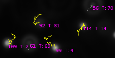
Draw Tracks: If this checkbox is activated all tracks are drawn on an ImageJ overlay. Yellow tracks have reached the minimum number of steps. Furthermore the size estimate followed by the track id is shown.
Size Distribution Estimation by Walker’s Method: If this checkbox is activated the size distribution is estimated by a maximum likelihood method described in [3]. The method exploits the fact that the mean squared displacements are gamma distributed. Please note, that the mean squared displacements used for this algorithm are measured indirectly. First, the diffusion coefficient D is estimated by the method specified in “Diffusion-Coefficient-Estimator”. Multiplying this diffusion coefficient by 4 and the framerate results in the corresponding mean squared displacement. If Walker’s Method is used, the result will only be a size distribution (no diffusion coefficient distribution)
Results
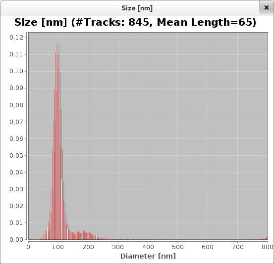
If the plugin finishes analyzing it opens histogram plots for the size distribution and the diffusion coefficient distribution. Please note that for calculating the distribution the track length is used as weighting factor. Furthermore the plugins open result tables for the histogram data (ideal for plotting with other software). The following plot shows a size distribution (using walker’s method & covariance estimator) estimated from a suspension with 100nm polystyrene beads (in water, 22C). The video used was captured with a nanosight LM10 microscope. The reported modal value is 98nm.
Simulation
If you like to check NanoTrackJ by Monte-Carlo simulation, you may use our simulation macros.
PartSimDC.ijm: This macro allows you to simulate particle by specifying their diffusion coefficient.
PartSimDia.ijm: This macro allows you to simulate particle by specifying their hydrodynamic diameter and a temperatur of the solution. Furthermore it allows to simulation polydisperse solutions by setting the number of particle qualities > 1.
Sample data
For the purpose of testing, you can download some sample video files.
NanoTrackJ settings which works well for this video:
| Parameter | Value |
|---|---|
| Center estimator | Maxima |
| Diffusion coefficient estimator | Covariance |
| Min. expected particle size | 90 nm |
| Search radius | 13.34 px |
| Min. number of steps per track | 20 |
| Temperature | 22,5 °C |
| Pixel size | 164 nm |
| Frame rate | 30 FPS |
| Linear drift corrected | True |
| Walker’s method used | True |
| Walker’s method min size | 800 nm |
| Mean size (Maxima Dialog) | 3 |
| Tolerance (Maxima Dialog) | 15 |
2. Video recording of freely diffusing 60 nm and 80 nm gold nanoparticles using dark field microscope
NanoTrackJ settings which works well for this video:
| Parameter | Value |
|---|---|
| Center estimator | Maxima |
| Diffusion coefficient estimator | Covariance |
| Min. expected particle size | 50 nm |
| Search radius | 18.03 px |
| Min. number of steps per track | 20 |
| Temperature | 24 °C |
| Pixel size | 182 nm |
| Frame rate | 25 FPS |
| Linear drift corrected | True |
| Walker’s method used | True |
| Walker’s method min size | 800 nm |
| Mean size (Maxima Dialog) | 4 |
| Tolerance (Maxima Dialog) | 12 |
References
[1] Ernst, D. & Köhler, J., 2013. How the number of fitting points for the slope of the mean-square displacement influences the experimentally determined particle size distribution from single-particle tracking. Physical chemistry chemical physics : PCCPs : PCCP, pp.3429–3432.
[2] Vestergaard, C. & Flyvbjerg, H., 2012. Optimal Estimation of Diffusion Coefficients from Noisy Time-Lapse-Recorded Single-Particle Trajectories. Technical University of Denmark.
[3] Walker, J.G., 2012. Improved nano-particle tracking analysis. Measurement Science and Technology, 23(6), p.065605.
[4] Van der Meeren P., Kasinos M., Saveyn H., “Relevance of Two-Dimensional Brownian Motion Dynamics in Applying Nanoparticle Tracking Analysis” in “Nanoparticles in Biology and Medicine”, Edited by M. Soloviev, Humana Press, New York, 2012