This page contains a tutorial for the MaMuT plugin. It describes and document all its features using a publication related dataset.
Publication
If you find MaMuT useful for your research, please cite it:
Installation
MaMuT is a Fiji plugin that depends on its components to run. Download Fiji from its website if you do not have it already.
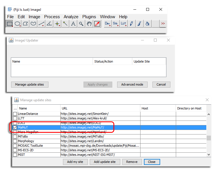
MaMuT is not shipped with Fiji by default; you have to install it in Fiji. Thanks to the ImageJ Updater, there is not much to do. Simply follow the instructions on how to follow a 3rd party site, and subscribe to the MaMuT update site. Here is briefly how to do it.
Got to Help › Update… and click on the Manage update sites button. In the window that appear, find the MaMuT checkbox and tick it. Then close the window. In the files to update list, there should be a plugins/MaMuT_.jar appearing. Click on Apply changes button, then restart Fiji.
Data preparation
MaMuT relies on and exploits the file format of the BigDataViewer. You need to prepare your images so that they can be opened in the BigDataViewer and there is no way around it. Actually, MaMuT was written specifically as an annotation platform for the BigDataViewer, specializing in cell lineaging.
If you already have such a file, skip to the next section. Otherwise, we lazily rely on the excellent BigDataViewer documentation and point directly to the BigDataViewer instructions to prepare your images, depending on whether
- they are opened as an ImageJ stack, or
- they come from a SPIM processing pipeline.
- they come from a new Multiview-Reconstruction datasets that are automatically in BigDataViewer format.
Once you have prepared your images for opening in the BigDataViewer, you should have a .xml file and a possibly very large .h5 file on your computer. The .xml file must be the output of the BigDataViewer data preparation. It should start with the following lines:
<?xml version="1.0" encoding="UTF-8"?>
<SpimData version="0.2">
  <BasePath type="relative">.</BasePath>
  <SequenceDescription>
    <ImageLoader format="bdv.hdf5">
      <hdf5 type="relative">MaMuT_Parhyale_demo.h5</hdf5>
...
Instead of preparing your own dataset, you can also download an example dataset for this tutorial here. In the following, we assume that you are using this data.
Opening and and saving in MaMuT
Starting a new annotation
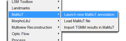
Start MaMuT on this dataset by browsing to Plugins › MaMuT › Launch new MaMuT annotation
A file explorer window opens. Browse to the .xml file of the BDV file pair. After a little while, the MaMuT main GUI window opens:
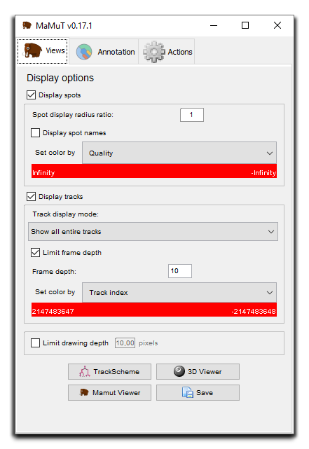
If you get this, so far so good. This is the main window of the GUI. It is split in 3 tabs but we will just focus on the first one for now. It controls the display of the data, both for the image and for the annotations. It also used to launch Views of the data. Right now there is no annotation data. We started by opening a BigDataViewer file, which is now loaded. The next MaMuT viewer (presented in the next section) you will open with display this image data, as in a normal BigDataViewer.
If you are familiar with the BigDataViewer, there is a few useful things to know. When we launch a new MaMuT annotation, we actually import some of the settings of the BigDataViewer in the session. For instance, in the BigDataViewer you can save and restore settings using the File › Save settings and File › Load settings menu item. This creates and loads a XML file typically named bdv_file.settings.xml if the BigDataViewer file is named bdv_file.xml. If this settings file is present in the same folder than the BigDataViewer file when launching a new MaMuT annotation, then MaMuT imports the brightness adjustments and bookmarks found in this file. The manual transformation and the groups are however not imported.
Saving to a MaMuT file
To save the annotation to a MaMuT file, press the Save button on the main GUI window. This will let you save to a file which is typically named bdv_file-mamut.xml if the BigDataViewer file was named bdv_file.xml.
The MaMuT files are actually TrackMate files. They are XML files with 3 main sections:
<?xml version="1.0" encoding="UTF-8"?>
  <TrackMate version="3.1.0">
    <Model spatialunits="pixels" timeunits="frames">
    <Settings>
    <GUIState>
...
The essential difference with plain TrackMate files is that the files generated by MaMuT have a Settings part that points to a BigDataViewer file as image source. Otherwise, the annotation stored in the Model section is described in the exact same way. So if you have a script that can load and analyse a TrackMate file, it is likely that it will also work with MaMuT.
In the last GUIState section, MaMuT stores several display settings. This is where you will find the brightness settings and the bookmarks location that we imported from the BigDataViewer settings when we launched the new MaMuT annotation and that you may modify later. From now on, they will be stored and retrieve directly from the MaMuT file, so the BigDataViewer settings file we used to launch the annotation is not used anymore.
So after saving, a MaMuT annotation is made of three files. In the case of the demo dataset:
MaMuT_Parhyale_demo.h5: this is typically a very large file that contains the raw image data.MaMuT_Parhyale_demo.xml: this is the BigDataViewer file. It is a XML file that lists where is the image data and how the possibly several views are arranged in space. This file can be opened in the BigDataViewer, and this is the one you open when you launch a new MaMuT annotationMaMuT_Parhyale_demo-mamut.xml: this is the MaMuT file. It contains as we said the the annotation and pointers to the image file.
From now on, we will only be interacting with the MaMuT file in MaMuT, but these three files need to travel together.
Loading a MaMuT file
To reload a MaMuT file, go to the Plugins › MaMuT › Load MaMuT file Fiji menu item, and browse to the MaMuT XML file. This will load the annotation and the image data. Careful, do not mix the MaMuT XML file with the BigDataViewer XML file when opening the later.
The MaMuT Viewer
MaMuT offers three kind of views:
- MaMuT Viewer is the main view that overlays the image data and the annotations using the physical coordinate system. This is where you will mainly interact with the data, and create, edit and move spots around. This view is based on the BigDataViewer.
- TrackScheme is the track browser, taken from TrackMate. It only shows the annotation data in a hierarchical way, discarding any physical location information. Tracks are laid out along time ranging from top to bottom, and arranged from left to right according to their name. This view is useful to make sense of the annotation data, as well as to edit links between spots.
- 3D Viewer shows a 3D View of the annotation data in the physical coordinate system, without the image data. It is based on the ImageJ 3D Viewer.
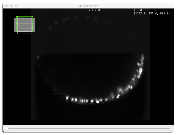
Let’s start with the MaMuT Viewer. Click on its button on the GUI, the one with a picture of a mammoth. A BigDataViewer window should appear.
The BigDataViewer framework and large, multi-view images
The MaMuT viewer is really a BigDataViewer window, so if you are familiar with this plugin, everything you know applies there. If not, here is a recapitulation of how the BigDataViewer works and how to interact with it.
A little word on the BigDataViewer: The BigDataViewer was made to deal with very large images of a sample possibly acquired from several different orientations (e.g. rotating the sample in a SPIM). These different orientations (or views, but here we use this word for another notion) of the data amount to a new dimension. This dimension if more complex to handle than e.g. multiple channels, because changing the acquisition orientation generates a data block which is not aligned with the other blocks (rotated, translated, and if you change the magnification, scaled), and does not have necessary the same size. As of today, only a limited numbers of image viewers can deal with multiple orientations, and the BigDataViewer is one of them.
Each of these orientations generate a data block, that we call source here. A source is monochromatic: if several fluorescence channels are captured under a single orientation, they each generate a source. The image data is not fully loaded in memory. It is cached efficiently following the caching strategy of the BigDataViewer (detailed here).
The tutorial dataset
The dataset we use for this tutorial is an excerpt from a long term time-lapse experiment done with a Zeiss LightSheet Z1, filming the development of a shrimp (Parhyale hawaiensis) over several days. We have here the first 10 time-points, spreading over a bit more than 1 hour. Three views were acquired that generated a source each:
- Angle 325° is the ventral-right view.
- Angle 280° is the ventral view.
- Angle 235° is the ventral-left view.
- Angle 0°, which is the first one in MaMuT, is the fused volume from all 3 input sources after spatiotemporal registration and multi-view deconvolution.
Exploring the data with the MaMuT viewer
Navigating through the data in space and time uses the mouse and keyboard in a standard way. Everything can be done with the mouse and keyboard. The key bindings can be redefined, but here are the default:
To pan and zoom:
 Right Drag or
  Middle Drag Move in the XY-plane of the view.
- Mouse Wheel Move along the Z-axis of the view. Press ⇧ Shift or ⌃ Ctrl to change the speed.
- ⌥ Alt + Mouse Wheel (Mac and Linux) or ⌃ Ctrl + ⇧ Shift + Mouse Wheel (Windows) Zoom in and out.
- ↑ Up / ↓ Down Zoom in / out. With ⇧ Shift fast zoom. With ⌃ Ctrl slow zoom.
To orient, rotate the view:
 Left Drag Rotate around the point where the mouse was clicked.
- X / Y / Z Select rotation axis.
- ↑ Up / ↓ Down Rotate clockwise / counter-clockwise around the chosen rotation axis.
- , / . Move forward / backward along the z-axis.
- ⇧ Shift + X Rotate to the ZY-plane of the current source (look along the x-axis of the current source).
- ⇧ Shift + Y or ⇧ Shift + C Rotate to the XZ-plane of the current source (look along the y-axis of the current source).
- ⇧ Shift + Z Rotate to the XY-plane of the current source (look along the z-axis of the current source).
To navigate in time:
- N Move to the previous time-point.
- M Move to the next time-point.
- [ Jump to the previous time step (explained below).
- ] Jump to the next time step.
There is a fantastic feature in the BigDataViewer that you will find here called bookmarks. They let you store a position and orientation in space as bookmarks. You can later call them again. To use them:
- First press ⇧ Shift + B then any other key to bookmark the current view position.
- Pressing B then the bookmark’s key to restore the view position.
- O does the same things, but only restore the bookmark orientation, and does not translate to its position.
You can many bookmarks, all identified by the key you press after the bookmark command.
Configuring the source visibility and display
Switching from one source to another is done with the numeric keys 1 … 0 for up to 10 views. Pressing F switches to the fused mode, where all sources are overlaid. You can add and remove sources from the fused view by pressing ⇧ Shift + 1 - etc. The color and brightness of each source are defined in the brightness and color panel, brought by pressing the S key.
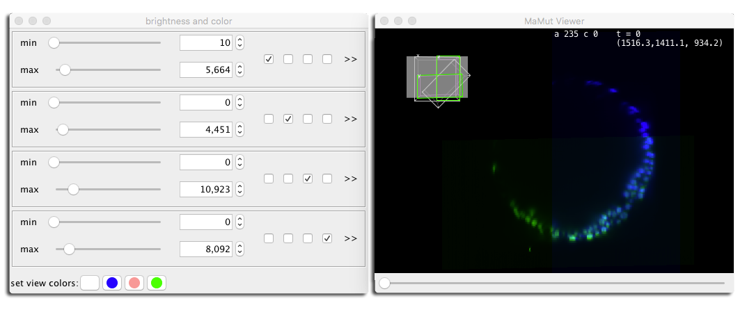
On this screenshot, we used the fused mode, toggle the first and third sources off (the deconvolved source and the angle 280°), and looked at the data in a XZ plane.
The MaMuT viewer also overlays some useful information:
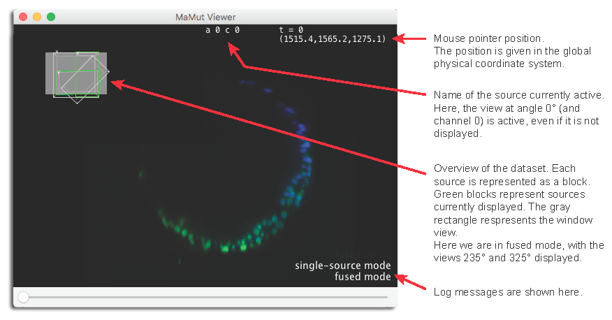
The MaMuT viewer only displays a slice of the current source(s). It fetches the pixel values it needs to generate a single slice through the data. By default, pixel values are interpolated using the nearest neighbor, which might generate a pixelated look for high level of zoom. By pressing I you can toggle between nearest-neighbor interpolation, and tri-linear interpolation, which smoothes the display.
Annotating cells
Creating spots
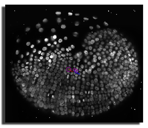
Using these commands, try to move the view around so that these cells are in sight.
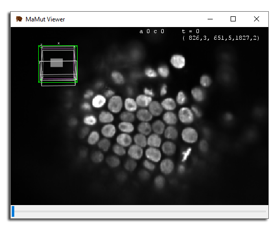
To do so, select the first source (angle 0°) and move the view in its XY place (press ⇧ Shift + Z). Then move in Z to the top of the embryo (around Z=1800) and finally zoom to bring about 50 cells in view. If you move in time, you can see that a lot of cell divisions are happening there. We will now build their lineage.
Move the mouse pointer over the cell you want to annotation, and press A. A magenta circle should appear, representing a cell or more generally, a spot. Spots are created, edited and removed using the following default key bindings:
- A to add a spot at the mouse location.
- D to delete the spot under the mouse location.
- Q / E to decrease / increase the spot radius. Use ⇧ Shift / ⌃ Ctrl to change the radius by a greater / smaller amount.
- ␣ Space is used to move a spot in the XY view plane: put the mouse pointer inside the spot you want to move, then press and hold space while moving the mouse. The spot will follow your mouse until you release the ␣ Space key.
Spots represents point of interest (in our case, cells) under the shape of a sphere. You can change the sphere time-point, location and radius, but that’s it. There is no object contour in MaMuT. Spots are drawn as circles in the MaMuT viewer, with the radius of their intersection with the view XY plane. If they are not intersecting with the view plane, they are drawn as small dots, as you can see by moving along Z a bit.
Using multiple viewers to position spots
Accurately placing a spot in 3D can be difficult. This is where using multiple views in MaMut can help. On the main GUI window, click on the MaMuT Viewer button again to open a new view. This new view might not be showing the spot you just added. Fortunately, all views can be brought in sync by clicking inside a spot.
In the first view, click on the spot you added. The second view is translated so that this very spot is brought at the center of the view window. Rotate around this point so as to show the YZ plane of the source (press ⇧ Shift + X) and zoom close to the spot, to have a view pair resembling this:
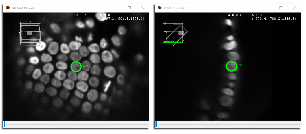
Just to ensure we are looking at the same spot in the two views, we checked the Display spots names button in the main GUI. Use the ␣ Space key to move the spot around in a plane until you are happy with its location. This view combination is useful to place properly spots in 3D. You can open as many views as you want. Other views can be used e.g. to have an overview of the data using a dezoomed view.
Spots can also be created with a double-click of the mouse. So if we recapitulate:
- Left Click inside a spot to select it and center all views to this spot.
- Double Click outside any spot to create a new one at the mouse location.
Display settings for spots
Now is a good time to talk a little bit on how we control the look of spots on the MaMuT viewer. All the MaMuT are in sync and they share common display settings. It is not possible to separately tune the display of each view. Display settings for spots can be tuned on the main GUI window, in the top part of the Views tab. Here you can toggle the visibility of all spots, make their name appear. The display radius simple change their apparent radius on the MaMuT viewer. This display setting has no impact on subsequent analysis and apart from visibility tidiness, it will have its utility later.
The spot colouring uses the notion of numerical features. In MaMuT, and as in TrackMate, each annotation object can have several numerical, scalar features associated. For instance a spot can have features like X, Y, Z for its position, etc. The drop-box menu Set color by lets you choose the feature you want to use for the spot color. The color range below the menu shows you the min and max value for the feature you picked over all the dataset and interpolate from blue to red with a jet color-map. If you scroll through the menu, you can see that the features available are sorted in three categories: spot features, default and track features. Spot features is the category where you can find all the numerical features that relate to single spots, like their position, radius, etc. In default, colours are not picked from a numerical feature, but either all the same (uniform color) or set manually (we will see later how). The track feature category is special: it gives to spots the color taken from the feature of the track they belong to.
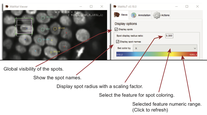
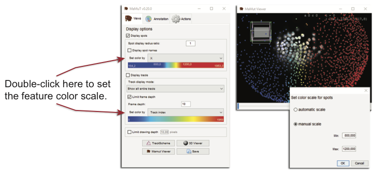
By default, the range of the color scale is taken from the minimal to the maximal feature value. This can be changed by double-clicking on the Set color by, which will bring a window where you can set the min and max manually.
Linking cells across time
The data structure behind MaMuT
We propagate the identity of a cell over time using several spots in several time-points, connected from one to its successor by links. Particle-linking algorithms are algorithms that find automatically what are the right links from one time-point to another given a set of spots spread over several time-points. Of course, the definition of “right” depends on the specificity of the algorithm. Tracking is the process of finding automatically all spots in an 2D+T or 3D+T image, and linking them. MaMuT does not do fully automatic tracking. It is a tool that specializes in manual or semi-automatic tracking, privileging data exploration and manual annotation on very large images. However, we will show in another tutorial how to import the results of automated tracking algorithms in MaMuT, so that they can be verified and curated. Here, we limit ourselves to manual and semi-automatic tracking.
A link is a directed relationship from a spot, called the source, to another spot, called the target. The source spot is always the predecessor in time, so links always point towards increasing time. All the spots that can be reached from a spot by crossing links form what is called a track. In our case, a track represents a lineage from a single starting (founder) cell.
The actual data structure behind the annotations in MaMuT (and TrackMate) is a simple directed graph. A graph is a mathematical structure made of vertices (in our case, spots representing cells) connected by edges (in our case, links representing propagation of identity across several time-points). The graph is simple because it is forbidden to have more than one link between two spots, and that a link cannot link a spot to itself. It is directed because links have a direction, following increasing time. In MaMuT, we added an extra constraint that forbids the existence of a link between two spots belonging to the same time-point, but otherwise this data structure is very standard.
So a link can be created between any two spots, provided they do not belong to the same time-point. There is no other restriction. For instance, a spot can be the source of several links. If there is two outgoing links from a spot, they may represent a cell division (mother cell linked to its two daughters). Several source spots can be linked to a single common target spot, though the biological meaning of this is less evident. MaMuT does not put constraints on the number of links going from or to a spot. We reasoned that MaMuT is to be used to build generic graph-like annotations, and that the subsequent analysis should be specific to the biological context. For instance, for cell lineaging there should be at most two outgoing links from a source spot, and at most one ingoing link on a target spot.
Creating and removing links
In the MaMuT Viewer, only spots are selectable with the mouse. To create or remove a link, you have to select exactly two spots.
- Select a spot by clicking inside it.
- Move to another time-point (N, M, [, ], the time slider).
- Add a second spot to the selection by shift-clicking inside it.
- Press L to add a link between these two spots, or to remove it already exists.
So here are the two new useful bindings for editing links:
- Shiftleftclick add and remove spots from the selection.
- L toggle a link between the two spots of the selection. This does nothing if there is not exactly two spots in the selection.
Now go back to your MaMuT session, with the data oriented as aid above, and try to annotate and link the cell that divides between the first and second time-point. The mother cell can be found around X=1095, Y=1020, Z=1820 and t=0. On the image below, we tracked the daughter cell that emerges from the division on the left part of the view.
![]()
Note that when you create a link with this method, after link creating the selection is set to be made of only the last spot added. To create the next link, you just have to add the target spot to the selection, the source spot is already in. But still, after creating links over only 10 time-points, let us admit that this is probably not the quickest way to quickly create a lineage. This method is probably best suited to edit an existing annotation.
The auto-linking mode
Press Shiftl with a MaMuT viewer window active. A message should appear in the MaMuT viewer that states the auto-linking mode is now on. In this mode, a link is automatically created when you create a new spot between this spot and the last one in the selection. Then the selection is changed to be the last spot added. Using this, you can quickly create lineage by moving forward in time with the keyboard and creating spots by typing A. You can also use Double Click to create spots, but because a simple click would clear the selection, you have to hold the ⇧ Shift key down to use auto-linking with mouse clicks.
Try to use the auto-linking mode to create the cell lineage of the dividing cell above, this time following the other daughter cell. Move back to the first time-point, select the mother cell, move to the second time-point M and add a spot A or Shiftdoubleclick on the cell location. Repeat by following the right daughter cell. You should end up with an annotation that resembles the following:
![]()
At this stage, your first track has two branches: the first cell at t=0 divides into two daughters, and each daughter makes a branch in the track. You do not have to specify to what track you want to branch from. Tracks are automatically merged and split when you add or remove links. The only editing you have to do is at the link level, and track are discovered from the spots connected by the links you created.
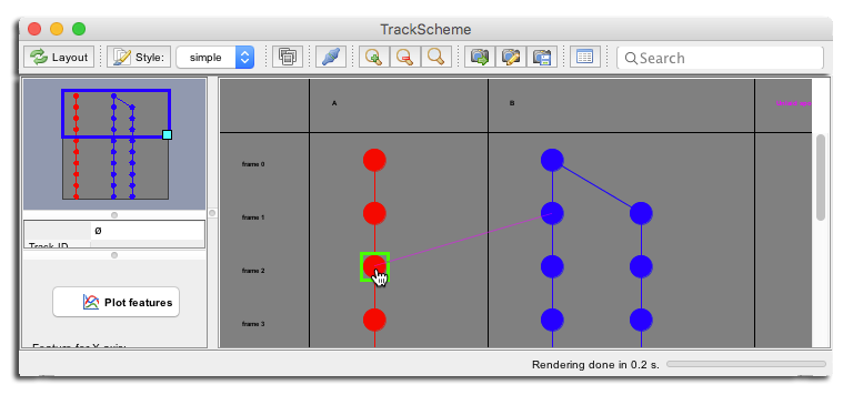
Step-wise time browsing and sparse annotations
MaMuT is built as an application for the annotation of large images immediately after their acquisition, and help build the first experimental results quickly. With modern, automated and fast live-sample microscopy, it is possible to generate a movie with high temporal resolution over a very long time. This is the case of the data we use for this tutorial, though we only work on the first 10 time-points. Nonetheless, you can see that at this stage, the cells move little from one frame to another. You could jump by steps of 5 frames, and still be able to identify the cell you tracked over time.
MaMuT has step-wise time browsing commands to just do that. The keyboard shortcut to do this are:
- [ Jump to the previous time step.
- ] Jump to the next time step.
By default, the viewer will jump to time-points multiples of 5: 0, 5, 10, etc. You can set what is the time step in the Annotation tab of the main GUI window, under the Stepwise time browsing field.
If you are on a time-point not a multiple of the time-step, the next key-press will move to the closest multiple. The goal of these commands is to quickly generate a lineage that extends deeply in time by skipping some frames. But the time-points we reach with these commands are always the same multiples, so the annotated frames are all the same when using the stepwise time browsing.
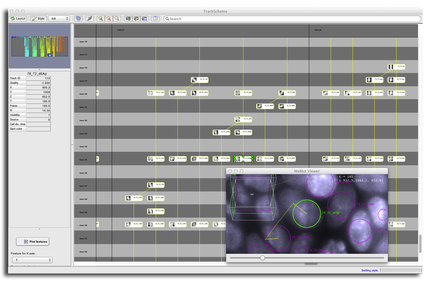
Below is an example from an actual annotation, peeking ahead the lineage visualizer we will describe in the next section. In this view, cells are arranged by lineage, time running from top to bottom. Time-points are lines of alternating color. You can see that except when cells are dividing or when there is an ambiguity, this user only annotated time-points multiples of 5. This leads to a sparser annotation, generated faster.
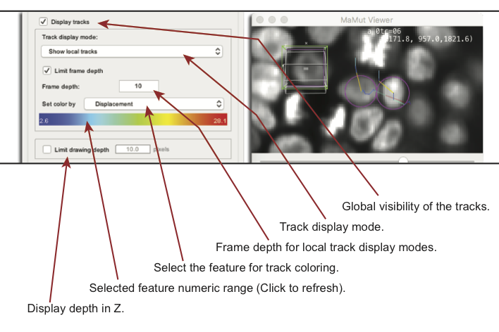
Display settings for tracks
Notice that the look of tracks (represented by a straight line for each link) can be tuned in the same way spots are.
Track coloring uses the same feature system than for spots. There are scalar numerical features associated to tracks and they are used to generate a color from a jet colormap. However, there is two kind of features for tracks:
- There are
track features, defined for whole tracks. For instance: the number of spots in a track, the displacement from the start to the end of track, etc. If you pick a track feature, all the links of a track will share the same color. - There are
edge features, defined for a single link. These are features that are simply defined by a link between two spots, for instance, the instantaneous velocity for the link. Then each link may be of a different color.
There is also a default category, like for spots, that allow for using a uniform color or to use link colors set manually elsewhere.
Tracks extend in time, and they are displayed as lines over the image data. By default, the whole tracks are displayed from their start to their end. You can control how they appear with the Track display mode menu:
Show all entire tracksis the default and display all the whole tracks with no time cue.Show local tracksonly shows a portion of the track which extend shortly before and after the current time-point. As the time distance increases, the track display fades in the image using transparency. You can control how much time context you want to display using the Limit frame depth checkbox and the Frame depth field.Show local tracks, backwardis similar, but only extends tracks backward in time (this mode is sometimes nicknamed ‘dragon tail’ in other softwares).Show local tracks, forwardis the same thing, but forward in time.- The same three modes are repeated with the
fastlabel added. They are identical to their counterparts, except that optimizations are made in favor of drawing speed, sacrificing frivolities such as transparency and anti-aliasing. - The last mode is
Show selection only, and only draws what is currently selected. It is very useful to make sense of a lineage amongst a possibly very large dataset. Careful: the content of the selection model can still be edited in this mode. For instance, if you click outside a spot, the selection is cleared and nothing will be displayed in this mode. This mode is best used in conjunction with TrackScheme, which we describe in the next section.
The Limit drawing depth field is used to restrict the Z neighborhood in which tracks are drawn. If activated, only part of the tracks that are close to the current Z plane of the view will be drawn. The extend of this Z section is set by the numerical value in the field.
TrackScheme
TrackScheme is the second view offered in MaMuT. It can be seen as a lineage visualizer or editor. In TrackScheme, the image data as well as the spatial location of spots are completely discarded in favor of a hierarchical layout that highlights how cells divide in time.
In the main MaMuT GUI window, click on the TrackScheme button. A new window should appear, with the following content.
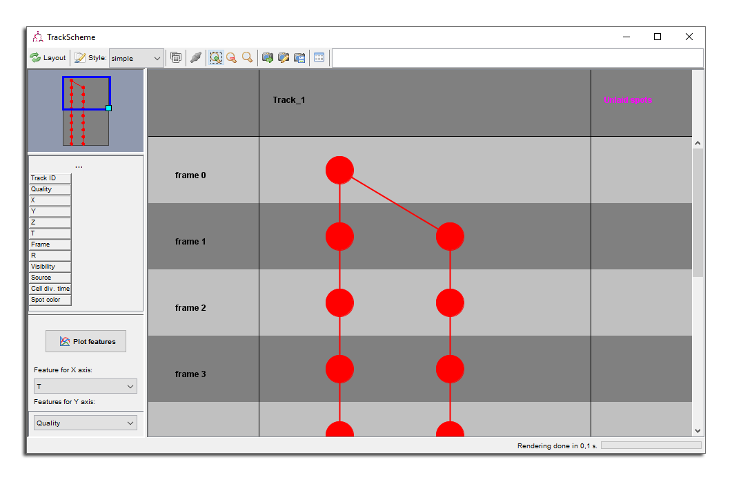
In TrackScheme, tracks are arranged from left to right and time runs from top to bottom. At this time we just have a single track, with two branches. The cell we tracked divides immediately after the first time-point, which is represented in TrackScheme by a fork going down. Each branch below this fork represents the annotation of a daughter cell. However, all the spots and links for these two daughter cells still belong to the same track, as they are connected via the mother cell.
Though this view is very synthetic, there is a lot you can do with TrackMate.
Moving around in TrackScheme
Moving around is done classically with the mouse, and the panning is triggered by holding down the ␣ Space key:
- Mouse Wheel scrolls up and down.
- ⇧ Shift + Mouse Wheel scrolls left and right.
- ␣ Space + Left Drag pans the view, à la ImageJ. If you pull the mouse out of the TrackScheme window, it will scroll in the direction of the mouse cursor.
- ␣ Space + Mouse Wheel is used for zooming.
The keyboard can also be used:
- The numeric keypad numbers 6, 9, 8, 7, 4, 1, 2 and 3 are used to move as on a compass.
- + zoom in.
- - zoom out.
- = restores the zoom to its default level.
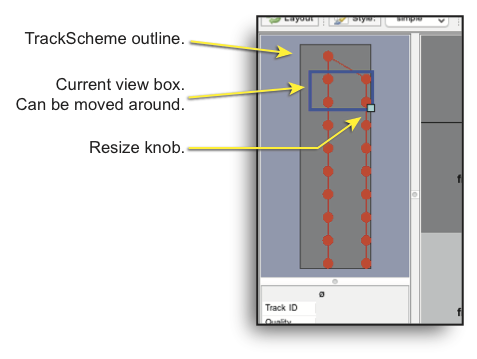
The top-left part of the TrackScheme window shows the outline of the graph. The blue square represents the current view and can be resized and moved around.
Configuring TrackScheme look
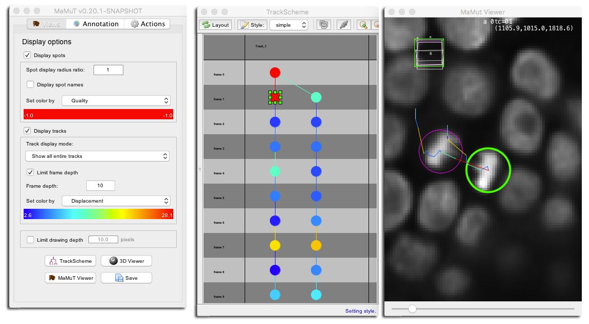
Though TrackScheme is a view of the annotation data like the MaMuT viewer, it completely and purposely ignores some the display settings you can set on the main GUI window, such as the track display mode and the global visibility of spots and tracks. The color it chooses for the links and spots representation is also peculiar: The spot color by feature mode is ignored, even for the circles that represent spot. They take their color from the track color mode, and use the color of the incident link. For instance, if you pick the Displacement feature in the track color mode, you will get this:
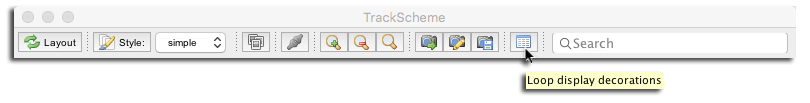
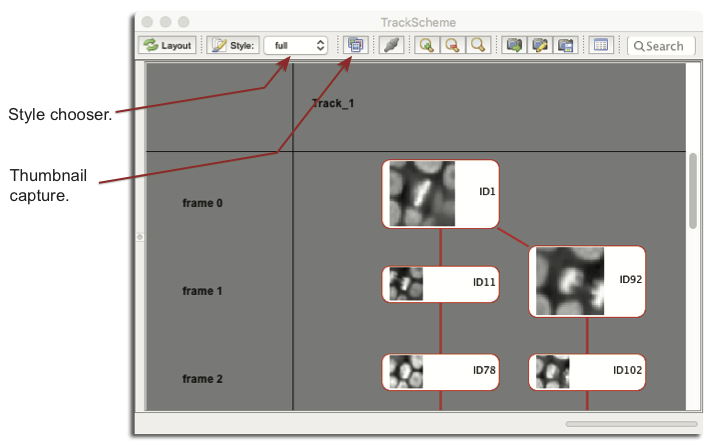
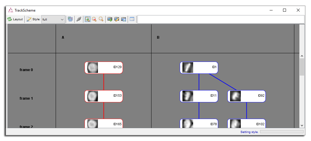
Tracks have a name, and are arranged in columns, separated by a vertical black line. TrackScheme arranges the annotations line by line, and each line represents a time-point. The row header tells you what time-point you are looking at. The background color of each row alternates to highlight different frames. If you find the background too crowded, you can disable the alternating color by clicking on the Display decoration button on the toolbar. The second mode disables track columns and rows alternating colors; the third mode re-enables track columns.
Finally, there is two Styles for the spot schemes. The simple style sonly displays them as round spots. The full style displays them as rounded boxes, with each spot name apparent. In the full style, small thumbnails can be captured and displayed in TrackScheme for all spots. Just next to the menu, there is a thumbnail button. If activated, thumbnails are collected from all spots, using the image source they were created on. Thumbnails are captured around the spot location, using their radius plus a tolerance factor. Interestingly, the Spot display radius ratio is used to define the size of the thumbnail. For instance, with a display factor of 2, you can obtain the layout below. Notice that the spot boxes can be resized manually to better display thumbnails.
Exporting TrackScheme display
The hierarchical layout of the lineages provided by TrackScheme can be useful for communications. It can be exported using the three export buttons in the toolbar.
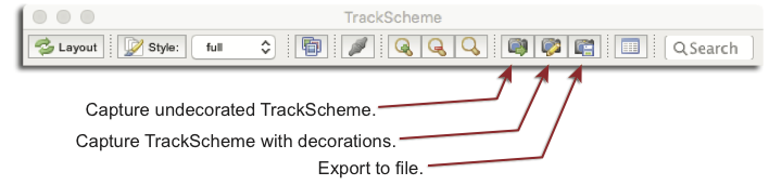
- The Capture undecorated TrackScheme button will generate a view of TrackScheme and open it in Fiji. The background is set to white and the zoom level is set to the default, regardless of what the actual zoom is in TrackScheme. Once this image is in Fiji, you can modify it, save it, etc using the tools in Fiji.
- The Capture TrackScheme with decorations button does the converse. It captures a snapshot of the TrackScheme window as is, and uses the current zoom level to generate an image.
- The Export to… opens file browser on which you can pick the export file format and its location. Many file formats are supported:
- PNG image file with/without transparent background.
- PDF or SVG file, that can later be edited with e.g. Illustrator.
- As a HTML page, though the layout is somewhat simplified.
- The now deprecated VML file format (replaced by SVG).
- As text, but this only saves a minimal amount of information.
- The MXE file format is a specialized XML format, that can be parsed with classical XML parsers.
- And all the common image formats (PNG, JPEG, GIF, BMP).
Managing a selection in TrackScheme
TrackScheme is useful to build a selection and query its properties. As we said above, TrackScheme does not abide any visibility setting. Spots and links are always visible, which is useful to build a selection. Spots and links are added to the current selection in a classical way:
- Left Click on a spot or link to set the selection with this spot or link. The selection is cleared before.
- Left Click outside a spot to clear the selection.
- ⇧ Shift + Left Click on a spot or link to add or remove this spot or link to the selection.
- Left Drag to select multiple spots and links in a selection box. Hold ⇧ Shift to add them to the current selection.
Adding to this, several items in the Right Click popup menu help selecting part of tracks. If you Right Click on a spot or Right Click outside a spot with a non-empty selection, you can:
Select whole trackwill include all the spots and the links of the tracks the selection belongs to.Select track downwardswalks from the spots and links in the selection, and add the spots and links that connect from them, forward in time (downward in TrackScheme).Select track upwardsdoes the same, but backward in time.
The same tools exist in the second tab of the main GUI window (Annotation), but we will speak of this tab later.
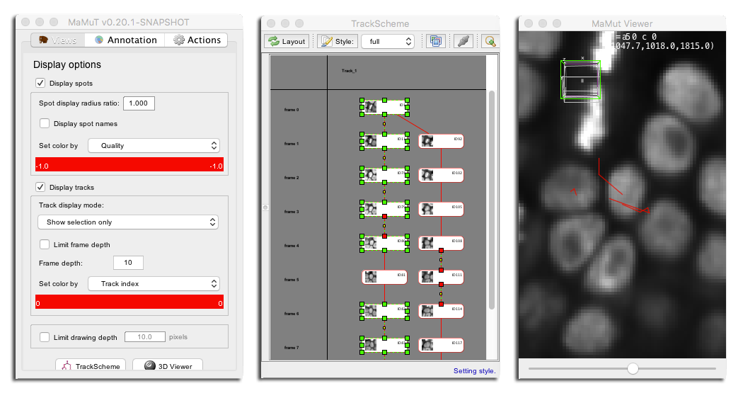
Selections are very useful for visualization within a crowded annotation. For instance, select one of the two branches in our single track. With the default track display mode, the selection is drawn on the MaMuT viewer as a thick green light that extends fully in time. The eighth track display mode is called Show selection only and just does that. It displays in the MaMuT viewer only the spots and links in the selection, with their proper color settings, and abide to the frame and depth limit settings.
For instance, you can use it to only display a series of disjoint parts of a tracks:
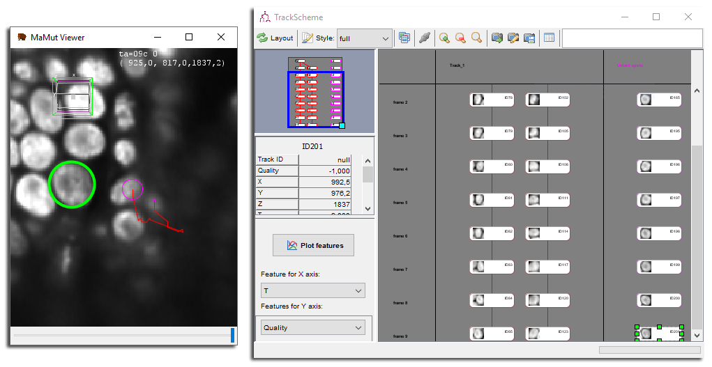
TrackScheme info-pane and feature plots
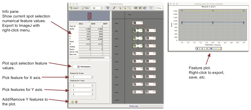
Another use of the selection is to display, plot and export information on its content. The left side bar of TrackScheme has two small panels dedicated to this, in addition to the outline panel in the top left.
The info pane in the middle left takes the shape of a table, that displays the numerical feature values of the spot selection as a table. Spots are arranged as columns and feature as lines. This table can be exported to an ImageJ table with the Right Click popup menu.
The bottom left part if the spot feature plotter. The Feature for X axis drop down menu lets you choose what will be the feature used for the X axis. Feature for Y axis menus work the same way. Y-axis features can be added and removed using the add and remove buttons.
To generate the plot, click the Plot features button. A graph should appear on which you can interact a bit. Left Drag towards the bottom right direction will zoom the plot, and Left Drag towards to up right direction will reset the zoom. The Right Click menu lets you configure the plot, save it to an image file and export it as an ImageJ table.
Editing annotations with TrackScheme
The main application of TrackScheme is to edit annotations in conjunction with creating and moving spots on another view. Let’s do this now.
Linking spots with the popup menu item
Make sure you have a TrackScheme window open, a MaMuT viewer window open, and move the later close to the cells we tracked previously. Make sure the auto-linking mode is off ⇧ Shift + L, and start creating spots over a cell close to the first one. Try to follow it over time. You should see spots appearing in TrackScheme, under a special column on the right called Unlaid spots. The TrackScheme window should resembles this:
Normally, TrackScheme only displays the spots that belong in a track. Lonely spots that are not linked to anything when you launch TrackScheme are not shown. The spots you create after TrackScheme are however stacked under this special column. From there, you can attach them to an existing track or create a new one.
Here is a way to do it. In TrackScheme using Left Drag select all the spots in the unlaid column. Right Click somewhere in TrackScheme to make the pop-up menu appear. One of the menu item should be something like Link 10 spots. Choose this one. Each spots is then linked to the next one, frame by frame, and the links should appear in TrackScheme and in the MaMuT viewer. You just created a new track.
Triggering re-layout and style refresh
Notice that the TrackScheme display of this new track is somewhat unsatisfactory. The first track may have changed color in the MaMuT viewer, but this change did not happen in TrackScheme. Plus, the new track does not have its own column, and the color of some of its spots might be wrong. The reasons for this are:
- We changed the annotation and these changes affected the numerical features that color the tracks. For instance, if you picked the
Track indexnumerical feature for track coloring, there is now two tracks instead of one. The feature update is seen immediately in the MaMuT viewer, but for performance reason, TrackScheme as well as the color line on the main GUI window have to be refreshed manually. To do so, click on the Style button in the TrackScheme toolbar, and directly on the track color line on the main GUI window.
- The changes we made affected the track hierarchy, but the re-layout is not triggered automatically by such changes. To do so, press the Layout button in TrackScheme toolbar. This will reorganize TrackScheme with a proper layout. Since in TrackScheme, spots can be moved around at will, this is also a good way to reorder things.
Linking spots with drag and drop
Another way to create single links is to enable the drag-and-drop linking mode. In the TrackScheme toolbar, click on the grated-out Toggle linking button.
Now move over any cell in one track. As you do, the cell gets highlighted with a green square. If you click and drag from this cell, a new link (in magenta) will emerge. Release it on any cells to create a link between the source and the target.
Removing spots and links
The last you link you added may have strongly perturbed our annotation, particularly if you did what was on the screenshot above. Correct it by removing the last link. Simply select it press ⌦ Delete. The same key will remove everything in the selection.
Editing track names and imposing track order
Tracks are ordered from left to right alphanumerically with their name. To change a track name, Double Click on it in the column header part. Track names should be made of a single line with a combination of any character.
Try for instance to change the track order by changing their name. Let’s call the first one ‘B’ and the second one ‘A’. Click the Layout button. Your TrackScheme window should look like this:
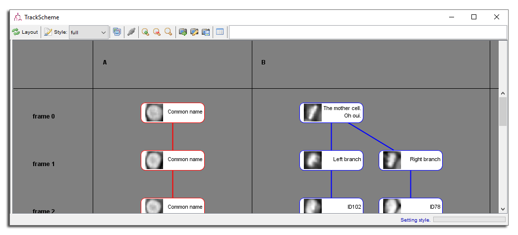
Editing spot names and imposing branch order
Spots also have a name, that you can see either in the MaMuT viewer by checking the Display spot names, either in TrackScheme by using the full display style. They are all called ID## by default, which is not very informative.
To edit a spot name in TrackScheme, Double Click on the spot. It should be replaced by an orange box in which you can type the spot name. Press ⇧ Shift + ↵ Enter to validate the new name, or ⎋ Esc to cancel the change. Spot names may be several lines long, but their display might then not be very pleasing.
You can also set the name of several spots at once. For instance, select the the whole second track (now named ‘A’) and Right Click (outside of a spot) to bring the popup menu. There is an item called Edit 10 spot names. The closest spot is changed to an edit box. When you validate the new name, all the selected spots get this new name.
Apart from their use to mark some biological meaning to the annotations, spot names have several uses. There is a search box in TrackScheme toolbar that centers the view on spots with name matching the text you enter there. Press ↵ Enter to loop over all the matching spots.
Spot names are also used to decide in what order to lay out track branches. For instance, our track ‘B’ as a cell division in the second time-point. You can force one branch to be the laid left or the right by setting the name of the spot just after the division. Sister cells are laid out from left to right alphanumerically, like for tracks.
Semi-automated tracking in MaMuT
MaMuT does not ship fully automatic detection and particle-linking algorithms. It was build as a tool for the manual annotation and inspection of large movies. Typically, you would use MaMuT just after the acquisition and image registration process, to check whether the data you acquired is usable, and quickly generate an annotation that will fuel your first scientific conclusions. Nonetheless, manual annotation can be very cumbersome. The semi-automatic tracking can alleviate this a bit.
Let us track one of the cell close to the two we just annotated. Go back to the first time-point and create a spot above a cell, with the right radius and location. In the main GUI window, click on the Annotation tab. You will notice that there is a Semi-automatic tracking panel. There are several parameters we will describe later. For now, simply change the Max nFrames value to 10, so that you get roughly this configuration for your TrackMate session:
![]()
Click on the spot you just added to add it to the selection, and click on the Semi-automatic tracking button. The tracking initiates and processes iteratively. Cells are discovered one time-point after the other, and added to track consecutively.
If you follow the case depicted above, the semi-automatic tracking does a mistake at frame 7. It captures a brighter, smaller cell further from its predecessor rather than the right one.
![]()
This gives us an opportunity to explain how does the semi-automatic tracking works and what are its limitations.
The semi-automatic tracking starts from a single cell in the selection. It inspects a neighborhood centered on this cell, but in the next time-point. The neighborhood is filtered by a Laplacian-of-Gaussian filter, tuned with the initial cell radius, and candidate cells are generated from the maxima in the filtered image. The filtered pixel-value of these maxima are used as a quality measure for candidate cell. The quality value is higher if the cell in the raw image is bright, and of radius similar to that of the initial cell.
Amongst these candidates, only those who have a quality higher than a fraction of the initial cell are retained. You set this parameter using the Quality threshold parameter in the Semi-automatic tracking panel. Only candidates with a quality larger than the quality of the initial cell times this threshold will be retained. Cells that are placed manually do not have a quality value (it shows up as -1 if you query it), so all the candidates cells are automatically accepted.
Candidates are then filtered by distance to the initial cell. Candidates that are found further away than Distance tolerance times the initial cell radius are discarded.
Then, amongst all the candidate cells that remain, the one with the largest quality value is accepted as a successor and linked to the initial cell. The process is then reiterated using the newly found cell as initial cell. The parameter Max nFrames allows to define a maximal number of times (and as such, of time-points) we iterate.
In our case, the error made at the time-point 7 was because there was a very bright cell that appeared in the neighborhood. Even if it was farther than the right candidate, it was within the Distance tolerance bound and was deemed as a successor. On this demo dataset, the temporal resolution is excellent, and the cells do not move much from one frame to another. A way to prevent the error we had would be to restrict the Distance tolerance to for instance 1.2 radius.
As we just saw, the semi-automatic tracking is very local and does not use nor derive any prior information on cell movements. It simple tries to find the best successor of a single cell, neglecting all the other cells. As such, it must be considered as a strongly suboptimal tracking method, whose goal is strictly to assist manual annotation. Alternating between semi-automatic tracking and manual annotation (e.g. using the auto-linking mode) when the semi-automatic tracking fails can generate deep lineages quickly.
Exporting images and reslicing data
Exporting the MaMuT viewer display
Notice that each MaMuT viewer window has a menu bar in which a few items are listed. You will find shortcuts to call for the help page, brings up the brightness and visibility dialogs, and in the Tools menu, the Record Movie and Record Max-Projection Movie commands. They are similar to their BigDataViewer counterpart, and were adapted so that the annotations are also visible on the exported images.
The Record Movie command will export a PNG capture of the viewer “as is”. All the source visibility and brightness settings are used, as well as the display settings for the annotation. Even the image size is taken from the current viewer window size. As only the current slice is exported, you can only configure the time-points to export.
Record Max-Projection Movie command performs a Maximum Intensity Projection of the data, in a direction orthogonal to the view plane. The annotations are projected as well, and they are drawn if they were located in the central slice. On the dialog of this command, you can configure how far from the current slice you want the projection to run, and how many slices to skip when doing the projection. Careful, the units used for this settings are in voxels, not in physical units.
Below is an example obtained on the last time-point of the demo dataset. Notice that the exported image a flattened view of the data, as RGB images.
Exporting a track sub-volume
Suppose you have now a very dense annotation that covers a large number of the cells in an already very large movie. Making sense of what happens to a single cell can be tricky given the density of information. A command in MaMuT lets you reslice the data to follow a small volume around a cell followed over time. It generates an ImageJ stack that follows the track over time, maintaining the tracked cell in the middle of the exported image.
First, select exactly two cells in TrackScheme or in a MaMuT viewer. These two cells must belong to the same track. We will export a volume that follows the cell over time, from the first to the second in selection by walking along a path that joins them in the track. For instance, select the first and last cell in the track now named ‘A’.
Once you have them, go the third tab in the main GUI window, called Actions. This tab contains only actions, that are MaMuT commands requiring special interaction with the data. Select the Export track stack action in the menu, and click the Execute button. A dialog shows up that allow configuring the export.
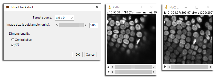
The dialog that pops let you choose first the source that will be resliced, in the Target source menu. Here we picked the first one. There is an important gotcha with the source selection and viewer orientation. The capture always uses the source intrinsic orientation. It will always capture Z-planes of the chosen source, irrespective of the view orientation in the MaMuT viewer. So if you capture the same track with two different sources, you might have very different orientation. The Image size field determines the size of the data exported, in units of the radius of the first select spot. Finally, the Dimensionality radio button lets you chose between exporting a 3D volume or just a single slice centered on the spot. In the example above, we generated the 3D volume following the track ‘A’, and on the left image, generated its maximal intensity projection.
This command really reads into the raw data, and therefore generate ImageJ stacks that have the same data representation (8-bit, 16-bit, etc) that of the raw data. This can be very useful for subsequent analysis.
Numerical features
We already skimed over numerical features when we discussed the display settings for spots and tracks. Numerical features are scalar values associated to a spot, a link or a track that measures some useful value. For instance, the X position of a spot, the displacement across a link, and the number of split events in a track. The MaMuT feature system is directly imported from TrackMate, and offers all the features available in TrackMate plus a few ones related to cell lineaging.
Numerical features are automatically kept in sync with the annotation. As soon as you add an annotation or modify and delete and existing one, the recalculation of features is triggered. As mentioned above however, the range display on the main GUI window is not, and you need to click over it to refresh the displayed colormap and its range.
The next paragraphs list and document some of the features in MaMuT.
Spot features
Quality |
The quality of the spot detection. This feature is normally created by spot detectors (such as the one used in the semi-automatic tracking), and relates to how likely the spot is to be relevant. By convention it is a positive number, and high values indicate good detection. Spot created manually have all a quality value equal to -1. |
X, Y & Z |
The spot location in the global common coordinate system. Units are whatever physical units used when creating the BigDataViewer file. |
T |
The spot time in physical unit. Units are whatever time units used when creating the BigDataViewer file. |
Frame |
The time-point in which the spot appears. |
Radius |
The spot radius, in physical units. |
Source ID |
The index of the source view in which the spot was created. For instance, if you created the spot with the first source active, then its source ID is 0. |
Cell division time |
This is a special feature made for cell lineaging. It is expressed in time units how long a the cell tracked by this spot takes to divide. The time is measured from the mother division to the daughter division, so the cell division time value will be the same for all the spots of a branch in a track. The branches that do not start with a cell division or do not finish by a cell division are excluded from calculation, and the value of spots that belong to such branches defaults to NaN. This is why if you use this feature in with our demo dataset to color spots, they will all be dark gray, as none of our tracks follow a full cell cycle. |
Manual spot color |
This is a special feature, that is not automatically calculated. You can assign manually a color to a set of spots. To do so, select some spots and in TrackScheme, right-click to show the pop-up menu. The menu item Manual color for X spots will let you set the selected spot color. This color will then be used in the views if you select the Manual color item in the Set color by menu in the spot panel of the main GUI window. Manual colors are saved to and retrieved from a MaMuT file. |
Link features
Spot source ID & Spot target ID |
The ID of the spot that is the source, respectively the target, of this link. In MaMuT and TrackMate, links have a direction, that follows time. |
Link cost |
The cost associated to the link. This value is normally set by particle-linking algorithms, that can create links between spots following minimization of global cost. Links created manually get a default value of -1. |
Speed |
The velocity calculated between the source and target spots, in physical units. |
Displacement |
The displacement calculated between the source and target spots, in physical units. |
Manual edge color |
Life for manual spot color, but for links. |
Track features
Track index & Track ID |
The track index and ID. Track index runs from 0 to the number of tracks. Track IDs are unique numbers generated for every new track. |
Duration of track |
The track duration in time units. Track duration is calculated from the earliest to the latest spot in time in the track. |
Track start & Track stop |
The track start and stop times. They are measured at the earliest and latest spots in the track. |
Track displacement |
The track displacement in physical units, calculated from the earliest to the latest spot in time in the track. Careful, this is not the maximal displacement in the track, just the distance between the first and last spot. |
Number of spots in track |
The number of spots in the track. |
Number of gaps |
The number of gap events in the track. A gap happens when a link is made between two spots separated by more than one frame. |
Longest gap |
The size of the largest gap in the track, in number of frames. |
Number of split events |
The number of split events in the track. A split event happens when a spot is the source to more than one link (but the target of at most one link). For instance, a cell division gives rise to a split event with two outgoing links. |
Number of merge events |
The number of merge events in the track. A merge event happens when a spot is the target to more than one link (but the source to at most one link). When several cell merges into one gives rise to a merge event. |
Complex points |
The number of complex points in the track. A complex point is a spot which the source to more than one link and the target of more than one link. |
Mean cell division time & Std cell division time |
The mean and standard deviation values of the Cell division time spot feature described above, averaged across track branches, and excluding undefined branch values. |
Customizing MaMuT viewer key-bindings
The mamut.properties file
The key-bindings used in the MaMuT viewer can be customized through a text file, that allow you to remap any command to any key. To so, create a text file named mamut.properties in the Fiji.app folder (where the plugins and jars folders are). This file must follow this syntax example:
A=add spot
ENTER=add spot
D=delete spot
E=increase spot radius
Q=decrease spot radius
shift\ E=increase spot radius a lot
shift\ Q=decrease spot radius a lot
control\ E=increase spot radius a bit
control\ Q=decrease spot radius a bit
...
It follows the syntax key=command, one per line. Modifier keys such as ⌃ Ctrl and ⇧ Shift are specified by prepending the key with their name, separated by a space escaped with a backslash ‘\’. Spaces in commands do not need to be escaped. The dash # character at the beginning of a line is used to insert comments.
An example of such a file can be found here.
Available commands
Here is a list of all available commands.
|
|
Add a spot at mouse location. If the |
|
|
Delete the spot at mouse location. |
|
|
Increase the spot radius at mouse location by 10%. |
|
|
Increase the spot radius at mouse location by 100%. |
|
|
Increase the spot radius at mouse location by 1%. |
|
|
Decrease the spot radius at mouse location by 9.10%. |
|
|
Decrease the spot radius at mouse location by 50%. |
|
|
Decrease the spot radius at mouse location by 1%. |
|
|
Add / Remove a link between two spots in the selection. |
|
|
Toggle the |
|
|
Launch semi-automatic tracking from the cells currently selected. |
|
|
Display the help window. |
|
|
Toggle the brightness settings dialog. |
|
|
Toggle the visibility and grouping settings dialog. |
|
|
Toggle interpolation method for pixel drawing between |
|
|
Toggle fused or single-source display mode. |
|
|
Toggle grouping mode. |
|
|
Replace X by a digit from 0 to 9. Toggle the visibility of the source X. |
|
|
Change the current view to align it with the XY planes of the source currently active. |
|
|
Change the current view to align it with the XZ planes of the source currently active. |
|
|
Change the current view to align it with the ZY planes of the source currently active. |
|
|
Move to the next time-point. |
|
|
Move to the previous time-point. |
|
|
Jump to the next time step. |
|
|
Jump to the previous time step. |
|
|
Store a bookmark for the current view. |
|
|
Move the view to the specified bookmark. |
|
|
Orient the view to the specified bookmark orientation. |
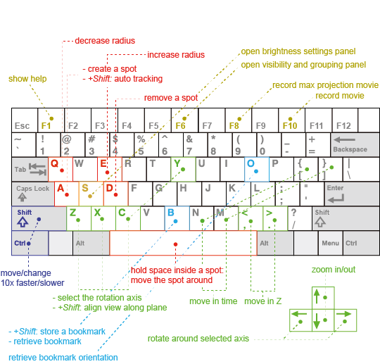
Default key-bindings
Here we recapitulate the default key-bindings for the MaMuT viewer. This image is also included in the help window of the MaMuT viewer.
TrackScheme key-bindings
TrackScheme key-bindings cannot be remapped like for the MaMuT viewer. We list them here.
|
F2 |
Edit current spot name. |
|
⌦ Delete |
Delete the current selection. |
|
↖ Home |
Center view on the first spot in current selection. |
|
↘ End |
Center view on the last spot in current selection. |
|
+ & = |
Zoom in. |
|
- |
Zoom out. |
|
⇧ Shift + = |
Reset zoom. |
|
1 2 ... 9 on the keypad |
Pan the view. |
|
⌃ Ctrl + A |
Select all. |
|
⌃ Ctrl + ⇧ Shift + A |
Clear selection. |
|
↑ Up / ↓ Down |
Move to the previous / next spot in time, within the current track. |
|
← Left / → Right |
Move to the previous / next sibling, within the current track. Sibling are spots that belong to the same track and to the same time-point. For instance the two spots of two sister daughter cells. |
|
⇞ Page Up / ⇟ Page Down |
Jump to the the previous / next track. |
|
⇧ Shift + |
Pan the view. |
|
⇧ Shift + |
Zoom in / out. |