This page describes how to visualize the various data sets provided as part of the Diadem Challenge in Fiji, and in particular viewing the traced neurons with Simple Neurite Tracer. The most important point about this is that the SWC files distributed as part of the challenge all use co-ordinates that are image-coordinates rather than world co-ordinates. (This isn’t how I interpret the paper that describes the SWC format, but in practice different software uses different conventions, so one has to deal with both.) This means that you should always select the “ignore image calibration” option when importing the SWC file into Simple Neurite Tracer. The other key point is that the image data are distributed with each slice in a separate TIFF file and don’t specify the slice separation in those files. So, after importing the sequence you will need to correct the calibration according to information on the Diadem challenge website or they will look odd when rendered in 3D. I describe these steps in more detail below.
If you have any comments or suggestions relating to this page, please email mark-diadem at longair dot net.
Olfactory Project Neurons
This data set is described here. I will go through loading the example “OP_1”. Each image stack in this data set is distributed as a directory of TIFF files, one per slice. To load such a stack, go to File › Import › Image Sequence and select the file “1.tif”. You should be shown a dialog like this:
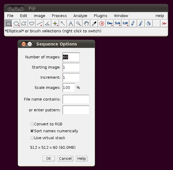
These default options should be fine - as you can see from the dialog it will have worked out that there are 60 image slices in that directory to be imported. If you click OK you should get a normal image stack:
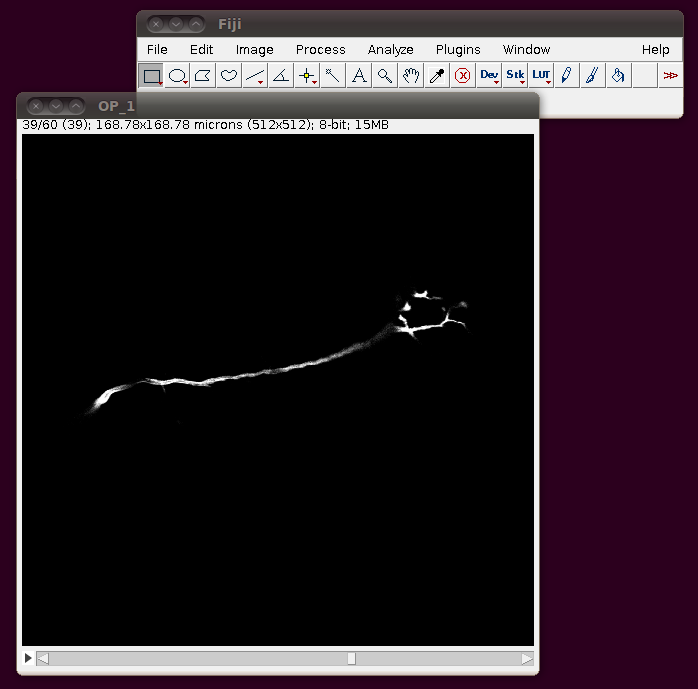
Unfortunately these TIFF files do not have the separation of these slices encoded correctly, so you should correct this manually. If you go to Image › Properties you will see that the pixel width, pixel height and voxel depth are all set to the same value (0.3296485). The page with information about the data set tells us that the z-separation should be three times the x and y separation, so correct the voxel depth to 3 times 0.3296485, like this:
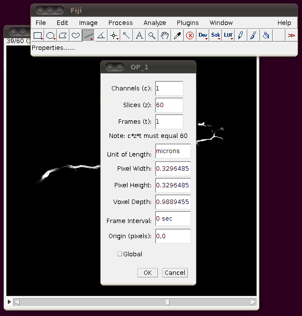
… and then press “OK”. To save yourself from having to re-enter this calibration information, and to be able to open the stack from the “Recent Files” menu, etc. I think it’s helpful to now save this stack as a single TIFF. So, I would go to File › Save As › Tiff … and save this as OP_1.tif in the directory above the one with individual slices.
Now start the tracing plugin by going to Plugins › Segmentation › Simple Neurite Tracer. If you keep the default options, you should see a display like this:
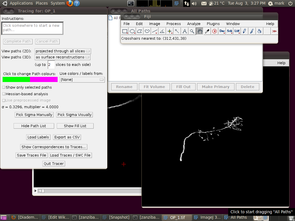
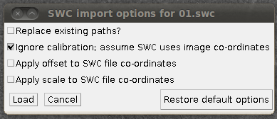
To load the SWC file with the supplied traces, click on “Load Traces / SWC File” and navigate to OP_1.swc. When you have selected this file, you will see the following options dialog:
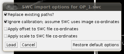
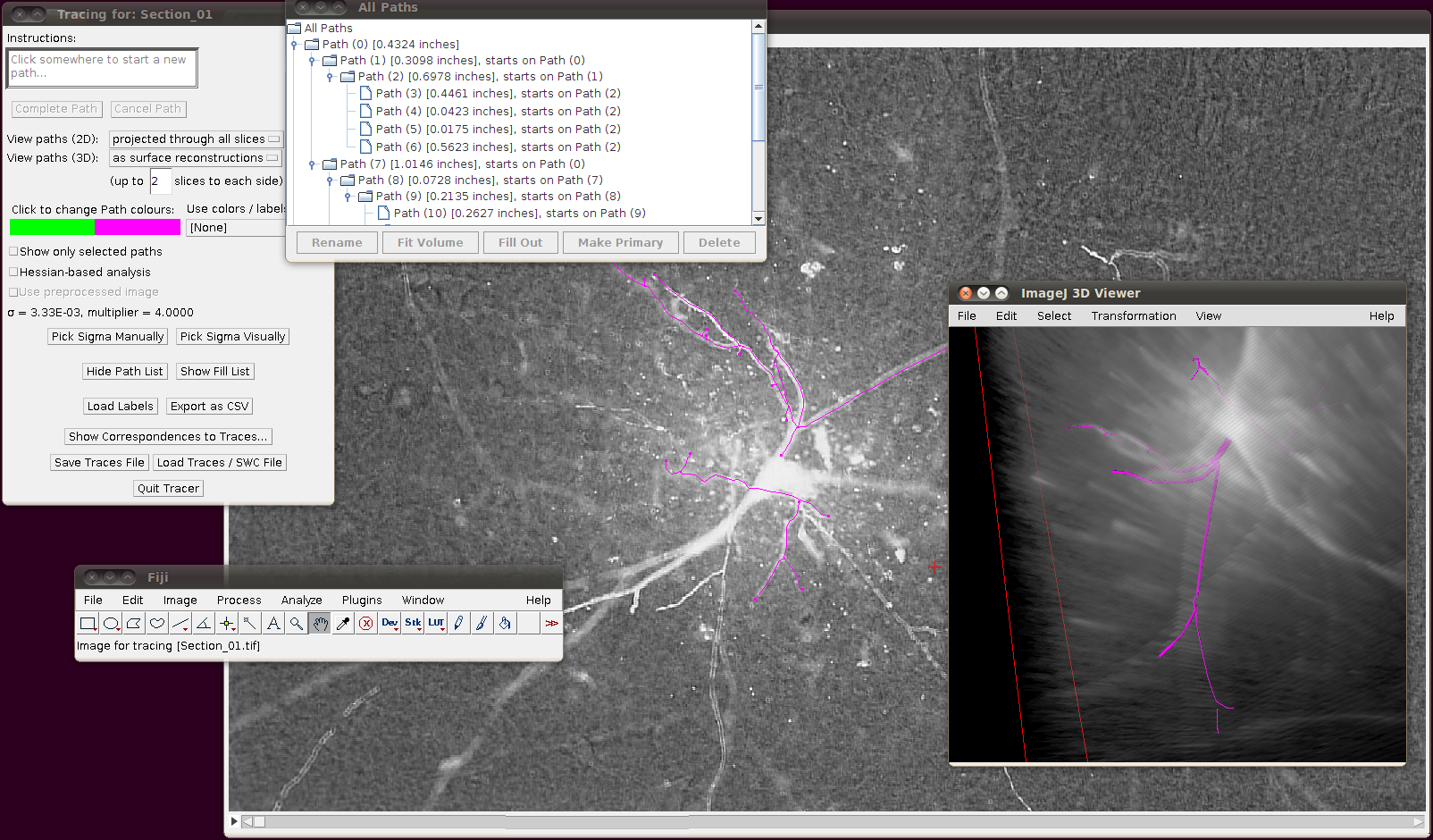
The important setting here is that you should have the “Ignore calibration” option selected. You should not apply an offset or scale for this data set. When you click OK you should see that the traces are overlayed in the stack window and in the 3D viewer:
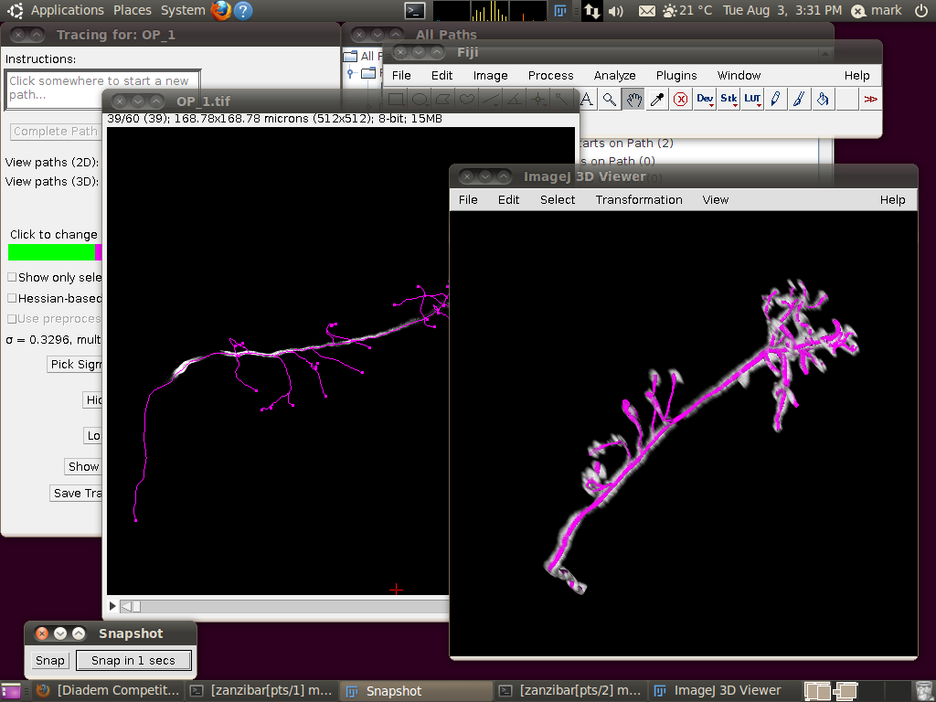
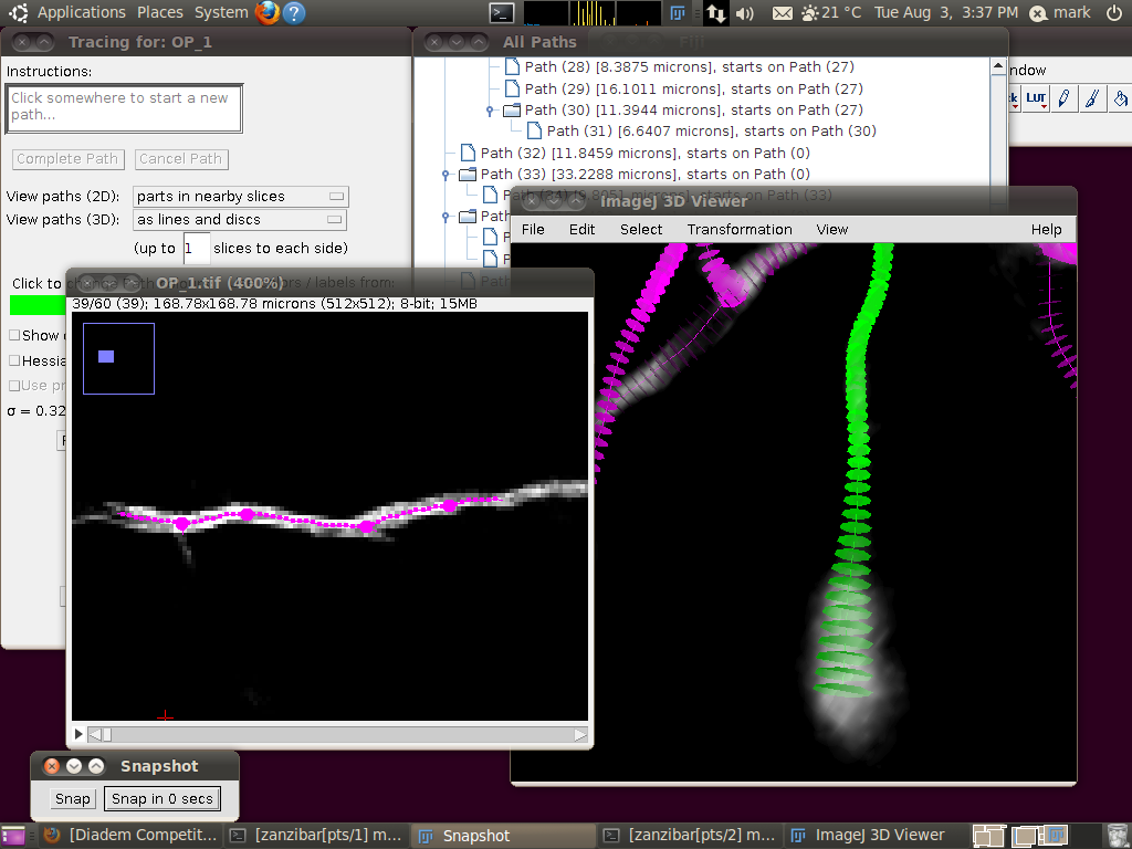
You may wish at this point to adjust the viewing options in the tracer’s dialog to examine the tracings in detail:
Diadem Neocortical Layer 1 Axons
The Neocortical Layer 1 Axons data set is based on a set of image stacks that need to be stitched together. The key point here is that you must use the offsets supplied by the Diadem challenge rather than allowing Fiji to stitch the automatically - the stitching will be subtly different.
Firstly, however, it will help to load each image sequence and save out the stack to a single TIFF image stack file. For each of the 6 directories, do the following: go to File › Import › Image sequence and select the first file in the directory (01.tif). After opening with the default options, save this out into the parent directory with the following names:
directory 01 -> Tile_01_02.tif
directory 02 -> Tile_02_02.tif
directory 03 -> Tile_03_02.tif
directory 04 -> Tile_03_01.tif
directory 05 -> Tile_02_01.tif
directory 06 -> Tile_01_01.tif
Now create a text file in the same directory called TileConfiguration.txt with the following contents, but changing the directory path to whereever these files are on your computer:
# Define the number of dimensions we are working on
dim = 3

# Define the image coordinates
/home/mark/diadem-examples/Neocortical/Tile_01_01.tif; ; (0.0, 0.0, 0.0)
/home/mark/diadem-examples/Neocortical/Tile_02_01.tif; ; (468.0, -14.0, -1.0)
/home/mark/diadem-examples/Neocortical/Tile_03_01.tif; ; (924.0, 3.0, -19.0)
/home/mark/diadem-examples/Neocortical/Tile_01_02.tif; ; (73.0, 507.0, -5.0)
/home/mark/diadem-examples/Neocortical/Tile_02_02.tif; ; (526.0, 484.0, 11.0)
/home/mark/diadem-examples/Neocortical/Tile_03_02.tif; ; (952.0, 462.0, -21.0)
These offset values are taken from the official page describing the data set.
Now you can stitch together the images using these offsets by going to Plugins › Stitching › Stitch Collection of Images, browsing to the TileConfiguration.txt file you’ve just created and making sure you uncheck the box “compute overlap”. It should look something like this:
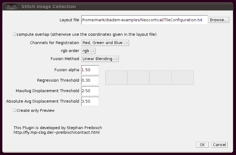
After clicking OK, this should stitch together all those stacks into one huge stack. (If there are problems, you should see details of them in the log window.)
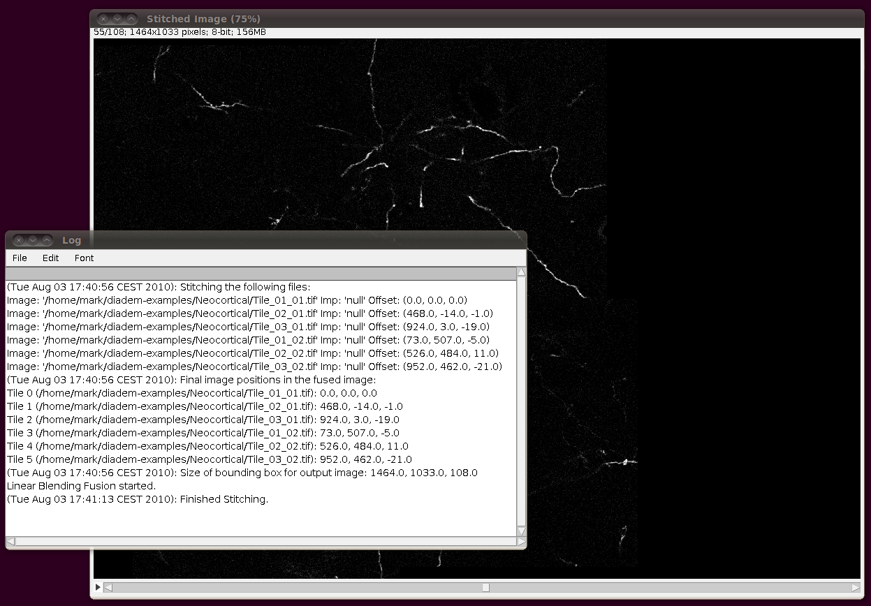
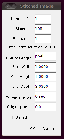
Next, you should correct the Z-calibration of the stitched stack. The data set page tells us that the z separation is 3.03 pixels, so open up Image › Properties and set the Voxel Depth to 3.03 times the Pixel Width:
Now you should save the stitched stack, and work from that from now on. (Since the stitched stack isn’t very large (156MB) one wonders why this wasn’t distributed already stitched.) Save the stack with File › Save As › Tiff….
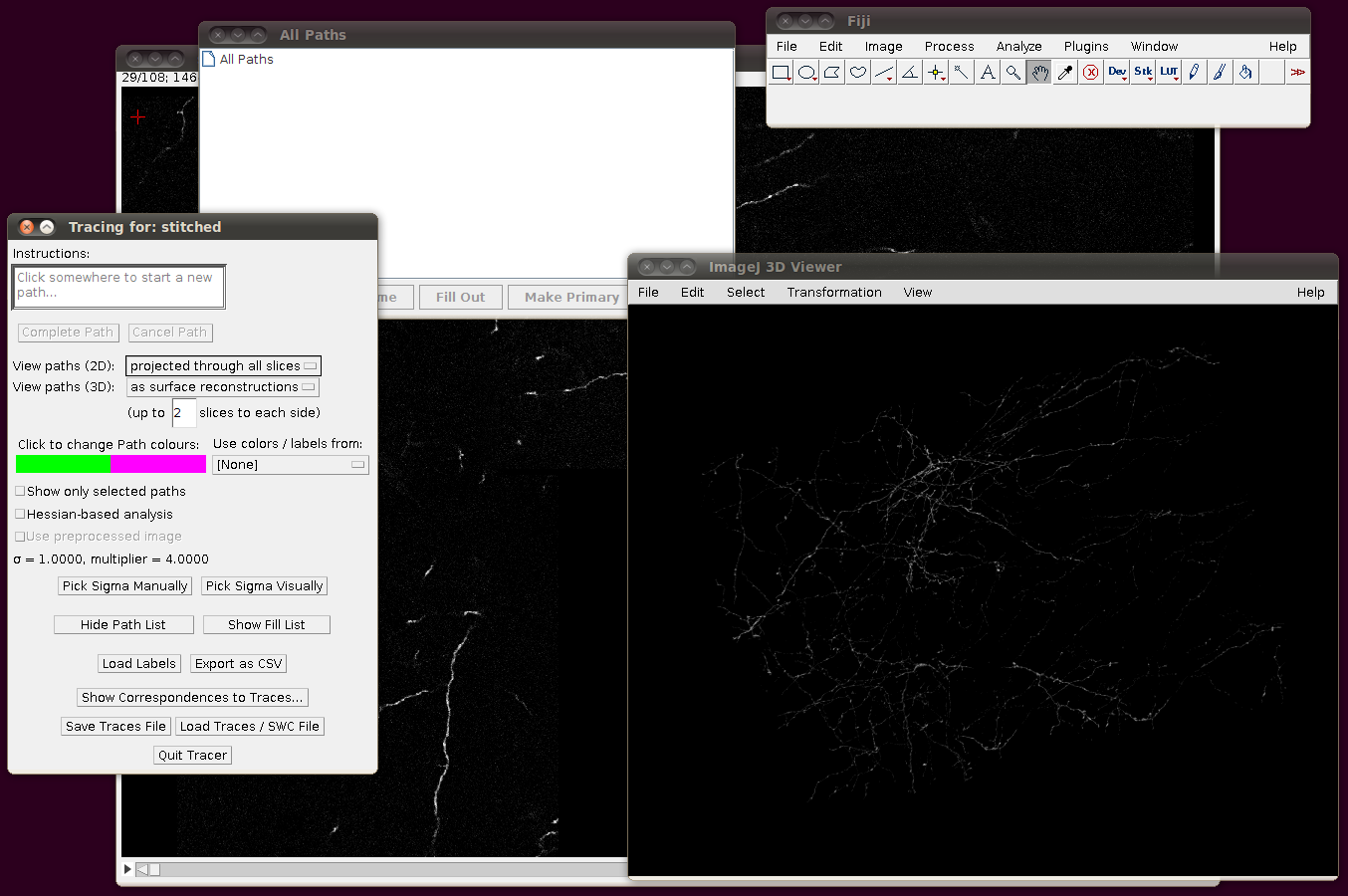
To load the SWC files, start up the tracer with Plugins › Segmentation › Simple Neurite Tracer. You should see something like this after it has started, with the stack rendered in the 3D Viewer:
You might have noticed that the offsets used in stitching above had some negative Y and Z values. This means that when you load in the SWC files, you will need to apply an offset to compensate for this. (0,0,0) in the stitched image will be at (0,-14,-21) in the space of the tracings, so when you click on “Import traces / SWC file” and have chosen (for example) NC_14.swc, you should expand the “Apply offset to SWC file co-ordinates” option and fill in these values:
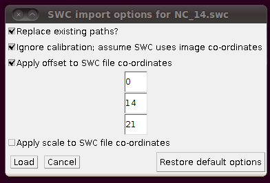
Then the traces should load in the correct position with those offsets:
Cerebellar Climbing Fibers
We will go through loading in the CF_1 image stack from the Cerebellar Climbing Fibers data set. The raw data for this image is stored in RGB and about 3.4GB in size, so for convenience you may wish to load this as a virtual stack (i.e. one where the slices are loaded from disk as required), convert it to 8-bit and resave the file first. In any case, I would recommend using a machine with 2GB of RAM (at the very least) to deal with these files.
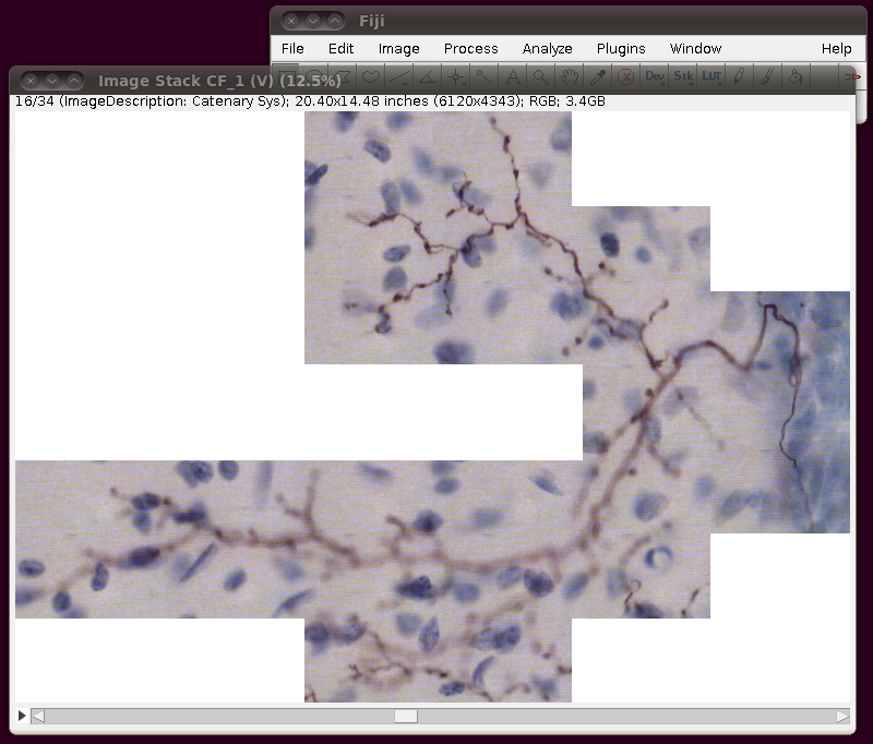
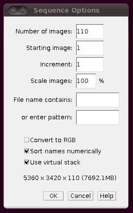
To load the files as a virtual stack, go to File › Import › Image Sequence … and select the first file in the sequence, “01.tif”. You will be presented with the import dialog, in which you should make sure that “Use virtual stack” is selected.
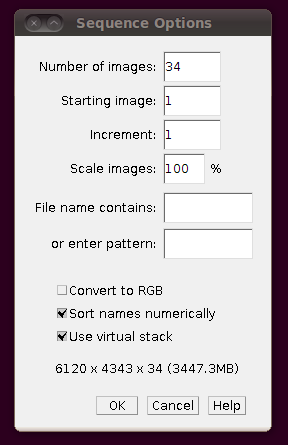
(Note that the number of slices in the directory (34) was automatically set.) You should now be able to browse through the stack:
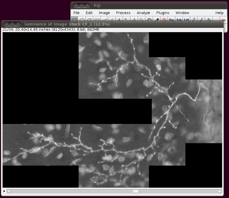
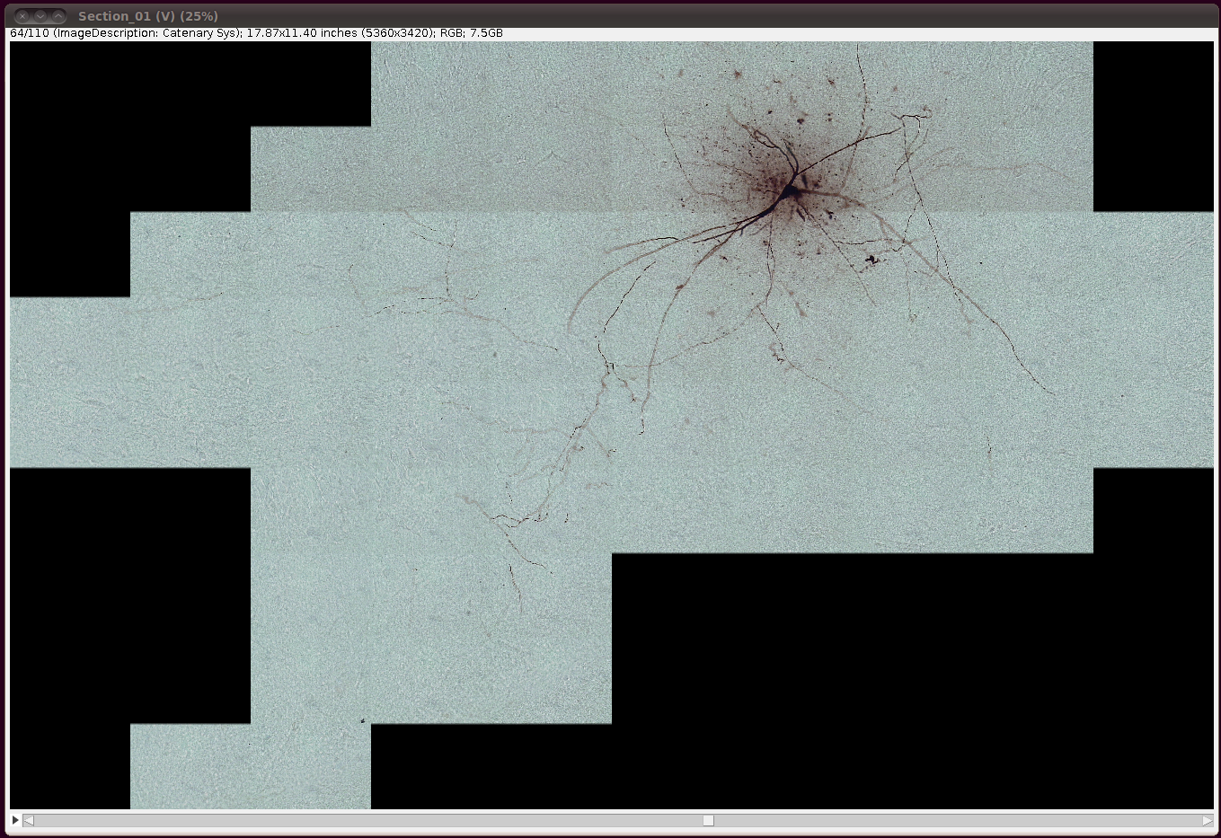
After loading this you need to convert this to 8-bit. You can do this in any number of ways, and if you’re actively working on a tracing task with this data you will probably want to do this in such a way that picks out the brown coloured neuronal processes. However, a simple way just for viewing purposes is to use the Image › Color › RGB to Luminance option. (Another option is to use Image › Type › 8-bit.) This will produce results like this:
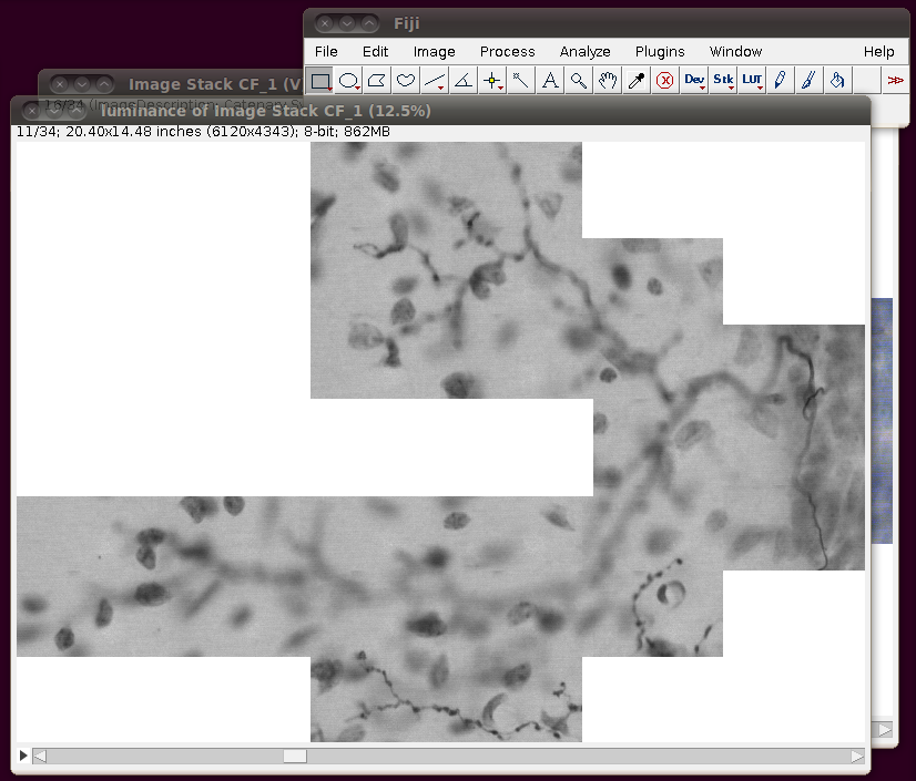
You can close the original virtual stack now.
It is a good idea to invert this image, since the 3D Viewer will make the low values of the image more transparent, and Simple Neurite Tracer assumes that neurons are brighter than their background. So, go to Edit › Invert and select “Yes” in response to the question about whether to process all 34 images. The results should look like this:
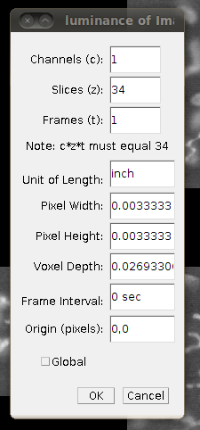
Before saving this out as a single 862MB stack, it is a good idea to correct the calibration of the image. The data set web page tells us that the separation between slices is 8.08 pixels. So, if you bring up the Image › Properties dialog, then you can correct the voxel depth to be 8.08 times the pixel width:
Now save this as a single TIFF stack called CF_1.tif by going to File › Save As › Tiff …, saving it in the directory above the one with the slices, to avoid confusion.
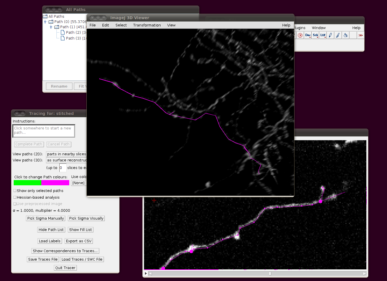
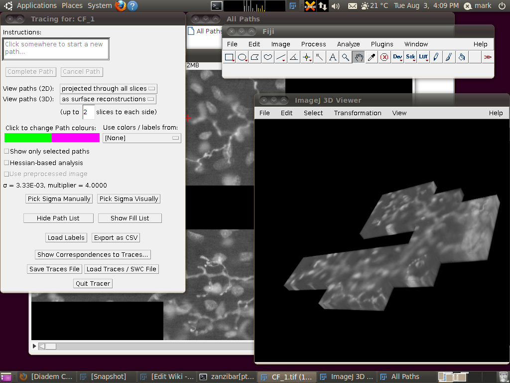
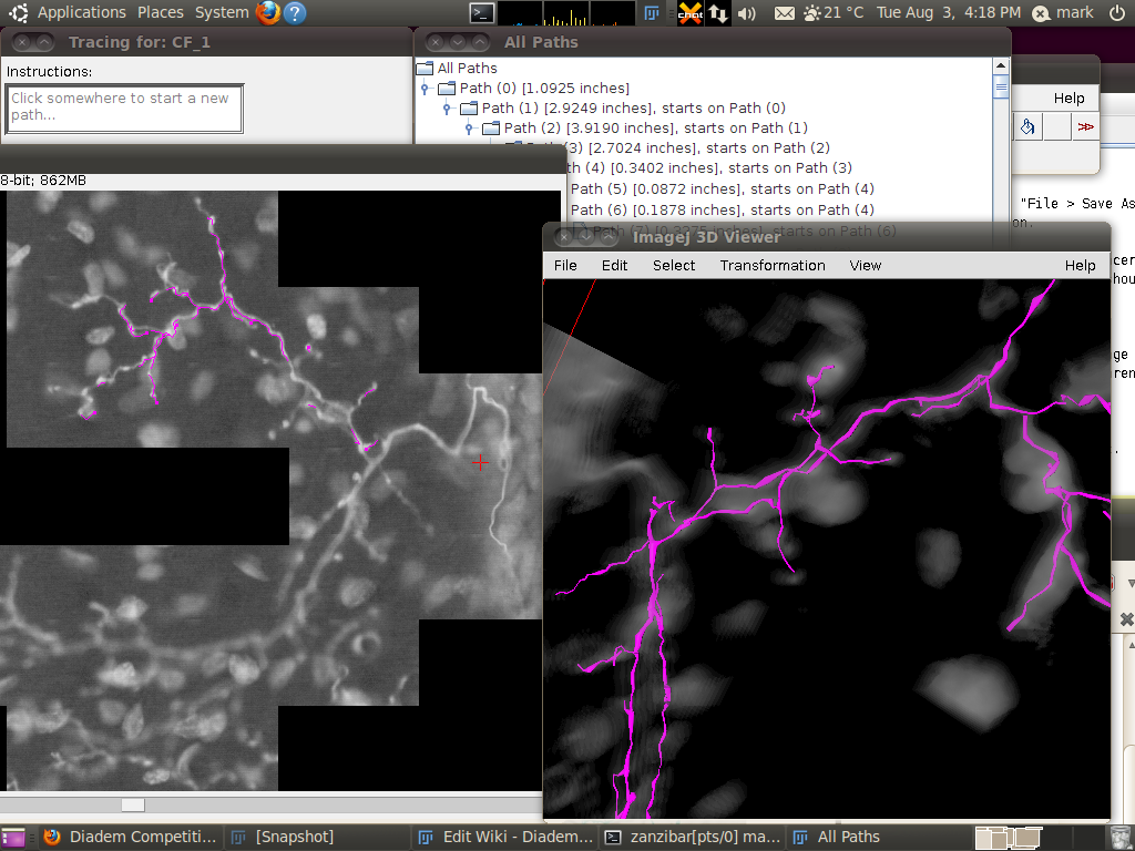
You can now start the tracer with Plugins › Segmentation › Simple Neurite Tracer. This may take some time, since there is a lot of data to load in to the 3D viewer. The result should look like this:
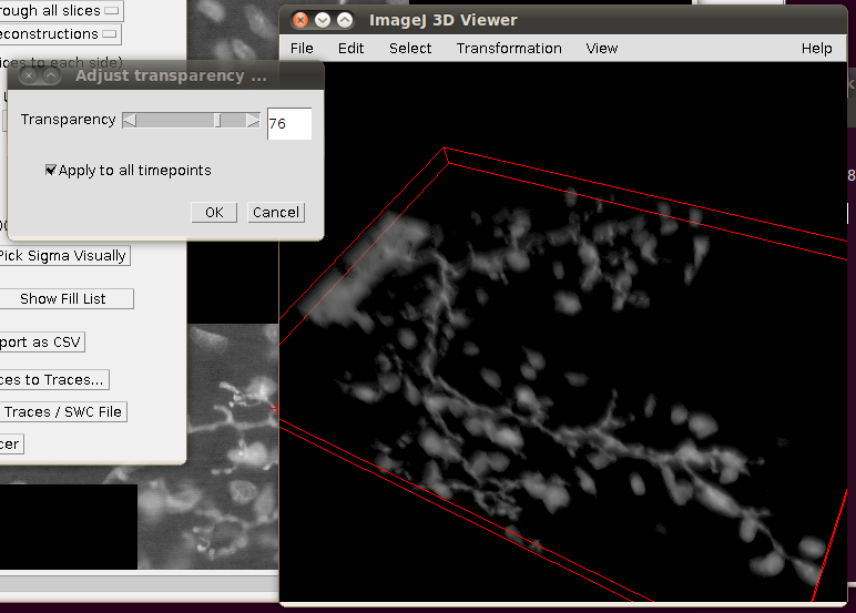
You may wish to adjust the transparency in the 3D viewer by selecting the image volume (left click on the image in the 3D viewer) and then going to Edit › Attributes › Change Transparency…:
Now, to load the traces click on “Load Traces / SWC File” and select CF_1.swc. You will be presented with an options box like this:
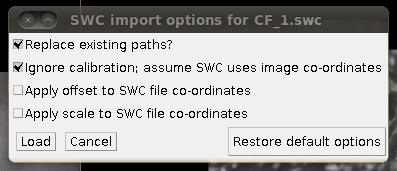
Make sure that “Ignore calibration” is selected (as in that screenshot) and that there is no offset or scale set. Once loaded you should be able to see the traces as here:
Hippocampal CA3 Interneuron
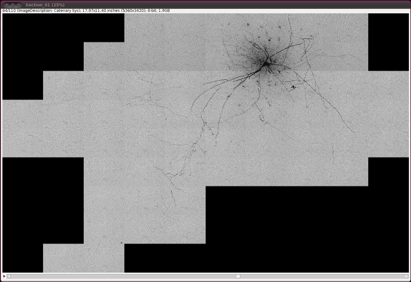
The Hippocampal CA3 Interneuron data set is difficult to deal with, since even after converting the stack to 8-bit values, it is still nearly 2GB in size.
As with the other stacks, you should load the image stack using Import › Image Sequence and selecting the “Use virtual stack” option:
That should load in the image data:
Now convert it to 8-bit with Image › Type › 8-bit. (The same comments as above regarding converting to 8-bit apply here as well.)
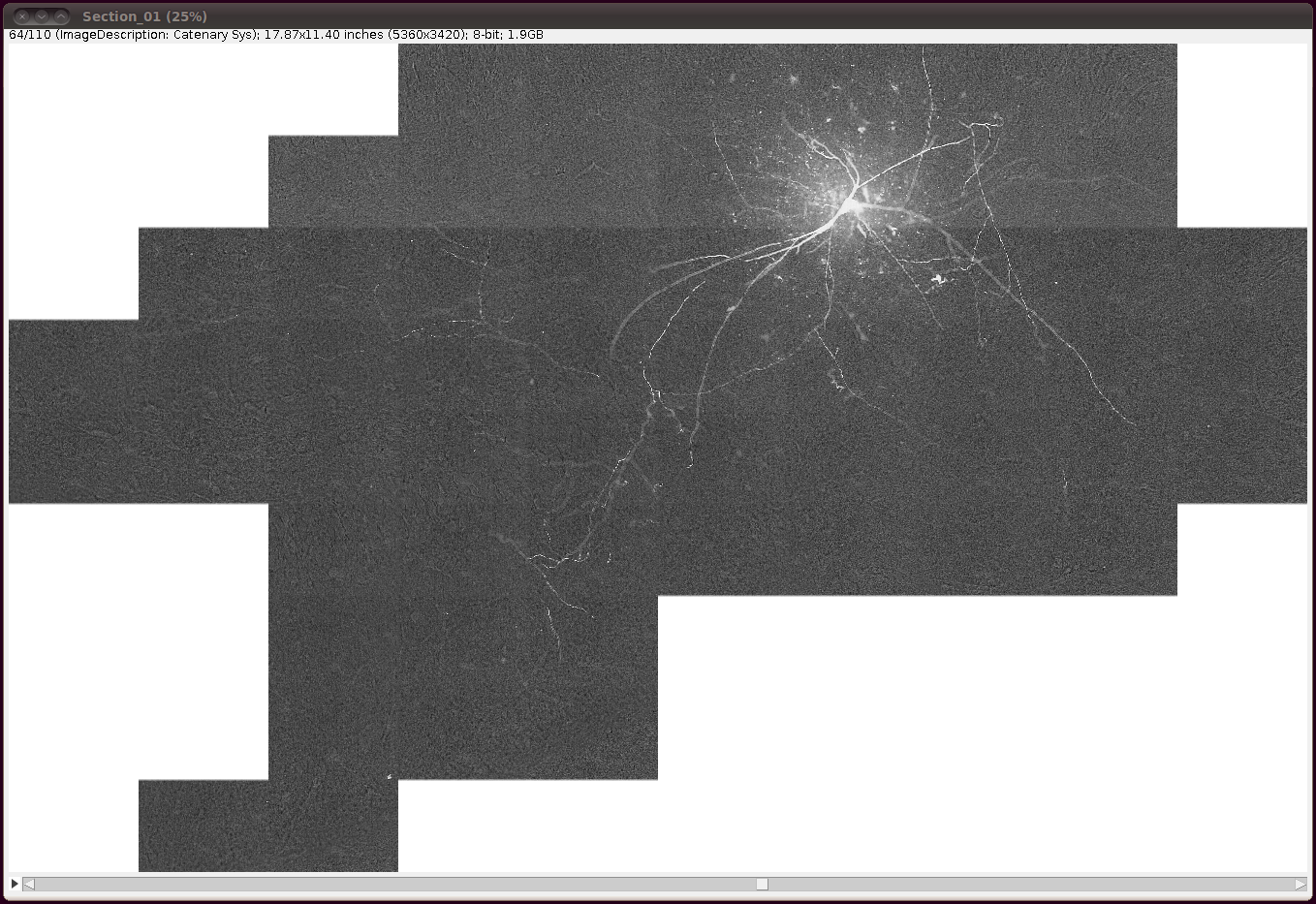
… and invert the image with Edit › Invert, saying “Yes” to the question about whether to process all 110 slices:
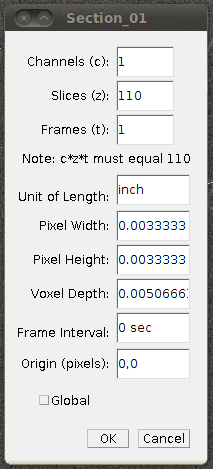
Now set the voxel depth to 1.52 times the voxel width, as specified on the data set page:
And then I would save this file as a TIFF stack (with Save As › Tiff…) so that you don’t have to go through these steps again. That will need about 2GB of disk space, and will only work if your filesystem supports single files of that size.
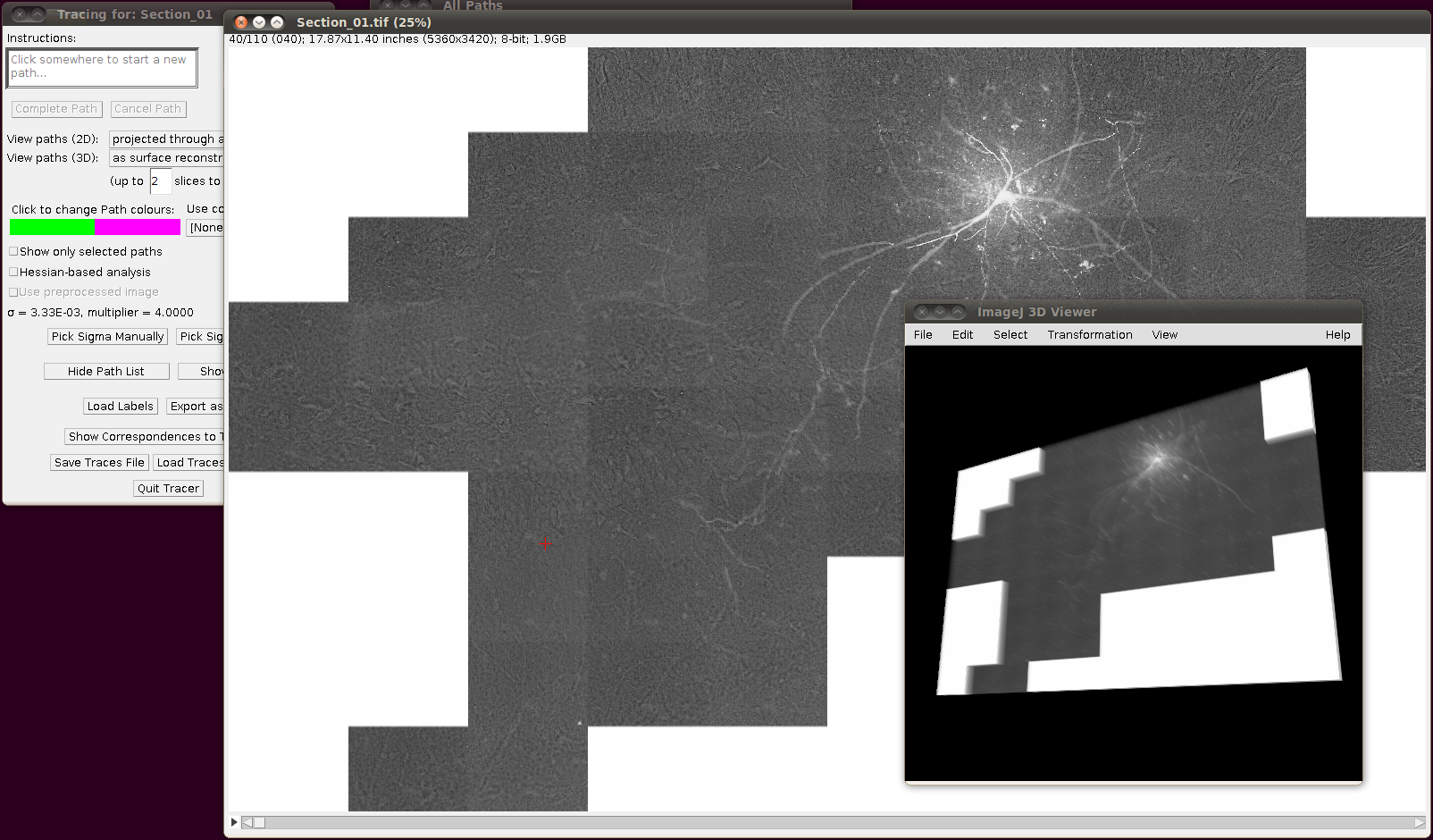
If you now start Plugins › Segmentation › Simple Neurite Tracer with its default options you should (eventually!) see something like the following:
Then you can load the SWC files via “Load Traces / SWC file” with these options:
(I’ve unchecked “Replace existing paths” for this data set, since it’s nice to load several SWC files into the tracer at once.) The results of loading three of the reconstructions, for example, might look like this:
Neuromuscular Projection Fibers
There are a number of caveats regarding these image data and reconstructions which are listed on its web page.
These 152 image stacks are in total so large that stitching them together and dealing with the stitched stack is not likely to be helpful. Instead, I would suggest that you just stitch together those images that you need to cover a particular SWC file. Since there are so many input stacks, I’ve written a clojure script for Fiji to help process these, which you can view and download via github. On running this script you will be asked to select a directory - you should select the directory that contains all of your unpacked image stack directories (probably called “000”, “001”, etc.) For each of these directories it will then:
- Import the sequence of slices
- Correct the calibration so that the voxel depth is 3.04 times the pixel width
- Write out each stack as a single TIFF stack (e.g. as well as the directory “000” you will also have “000.tif”
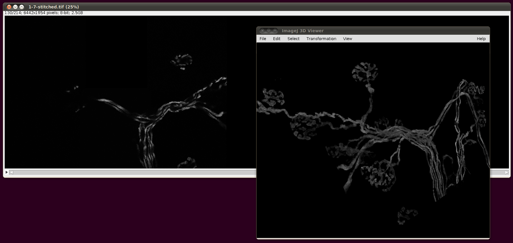
Finally, the script will output a TileConfiguration.txt file in the same directory. Supposing one had vast amounts of RAM, this file could be used unaltered with Plugins › Stitching › Stitch Collection of Images, as above. However, the file is still useful even with modest amounts of RAM, since you can copy this file to a new name and edit out all but a few of the images that are listed there. For example, here are image stacks 000 to 007 stitched together:
That script may be useful as a basis for a smarter selection of images to stitch for particular reconstructions.
You should then be able to adjust the SWC import options in order to import the reconstructions in the correct positions - you will need to understand the translations described for the reconstructions on the web page in order to get this right. (I haven’t had time to do this accurately myself yet.)